3.2.3. Thresholding
Visual inspection of a lot of images reveals that the objects of interests (the coins in the image below) have a gray value that is different from the background. In these cases the histogram will often show a bimodal distribution.
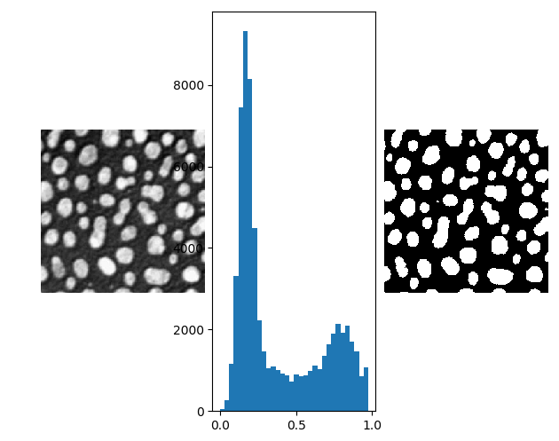
In the above image showing particles embedded in a substrate, the particles are brighter (more white) than the background. This is also clearly visible in the histogram. On the right in the above figure the thresholded image is shown. The threshold value is manually selected at \(t=0.5\).
There are many algorithms known that automatically calculate a suitable threshold for an image. In this section we will only look at one of them.
3.2.3.1. Isodata Thresholding
Isodata thresholding is a way to automatically find a threshold for a given gray value image \(f\). Consider a threshold \(t\) somewhere in the range of gray values in the image. Then we consider the mean of all pixels in the image with a gray value less then or equal to \(t\), call it \(m_L\) and the mean of all pixels with gray value greater than \(t\), let’s call that \(m_H\).
Isodate thresholding then finds a threshold such that
i.e. the value of \(t\) is such that \(t\) is halfway inbetween \(m_L\) and \(m_H\). Please not that both \(m_L\) and \(m_H\) are functions of \(t\). Therefor the above equation can be written as
defining the function \(m\). A point \(t\) such that \(t=m(t)\) is called a fixed point of the function \(m\). Starting from an initial estimate \(t_0\) the fixed point can be found with fixed point iteration:
In python this would result in the following code:
In [1]: f = plt.imread('images/cermet.png')

In [2]: t = 0.2

In [3]: epst = 0.01

In [4]: while 1:
   ...:     mL = f[f<=t].mean()
   ...:     mH = f[f>t].mean()
   ...:     t_new = (mL+mH)/2
   ...:     if abs(t-t_new) < epst:
   ...:         break
   ...:     t = t_new
   ...:     print(t)
   ...:
0.3491027355194092
0.45121729373931885
0.480459988117218
The threshold value that is calculated is \(t=0.488\) and close to what we had manually selected.
In an exercise you are asked to implement the isodata thresholding algorithm using the histogram data instead of accessing all pixels in the entire image in every iteration.
3.2.3.2. Exercises
- The isodata threshold algorithm was implemented in a previous
section using the image directly. This obviously is overkill. We
don’t need all individual pixel values, all we need is the
histogram of the image.
- Given a histogram
hof the image. The mid points of the bins are in arraym. Give the expressions to calculate \(m_L\) and \(m_H\) as used in the isodata algorithm. - Implement the isodata threshold algorithm using the histogram
and not the individual pixel values (once the histogram is
calculated of course). Note that
epstshould be related to the bin width of the histogram.
- Given a histogram
- It is not that hard to prove that the isodata threshold algorithm
really is 2-means clustering in disguise.
- Can you prove that?
- Using k-means clustering we can try to find more than just a background and object cluster. This might be usefull to segment images where more than two dominant gray values are present.
- Formulating thresholding as 2-means clustering also opens the possibility to ‘threshold’ color images directly without first looking at just the luminance values.