1.7. Some Bits of Information Theory

1.7.1. Entropy

Information is linked to probability: an unlikely event is associated with a high information content. Claude Shannon was the first to give a solid mathematical model for this intuition. For an event \(A\) with probability \(P(A)\) he defined self information

\[I(A) = -\log_b(P(A))\]

An event with probability one has zero self information. Nowing that it will rain every single day does not really provide any information. An event with very low probability is so rare that in case it does occur carries with it a lot of information. Note that an event with \(P(A)=0\) is not really an event in the sense that it will never occur. In information theory we will only consider events for which \(0<P(A)\leq 1\). For events that are very unlikely, i.e. \(P(A)\ll 1\), the self information is very high. It is a very rare event and if such an event really occurs the information is high.

The unit of self information depends on the choice for the base \(b\) of the logarithm. For \(b=2\) we express the self information in bits, for \(b=e\) we use nats and for \(b=10\) we use decimals. From now on we will use \(b=2\). Note that bits in this definition are not bits as we know in computer science (but related).

Consider a discrete random variable \(X\). The expected self information in observing one value is called the entropy of \(X\) and can be calculated with

\[\begin{split}H = E(I(X=x)) &= \sum_{x} I(X=x)\, P(X=x)\\ &= - \sum_{x} P(X=x) \log_2 P(X=x)\end{split}\]

Consider a uniformly distributed random variable with probability function \(p(x)=P(X=x)\):

\[\begin{split}p(x) = \begin{cases} \tfrac{1}{8} &: 1\leq x \leq 8\\ 0 &: \text{elsewhere} \end{cases}\end{split}\]

The entropy for this distribution is \(H=3\, \text{bits}\). Note that this number is equal to the number of computer bits needed to encode a number in the range from 0 to 7 (i.e. 8 different numbers).

Now consider a random variable with probability function

\[\begin{split}p(x) = \begin{cases} \tfrac{1}{2} &: 1\leq x \leq 2\\ 0 &: \text{elsewhere} \end{cases}\end{split}\]

For this distribution the entropy is

\[\begin{split}H &= -\tfrac{1}{2} \log_2(\tfrac{1}{2}) - \tfrac{1}{2} \log_2(\tfrac{1}{2})\\ &= \tfrac{1}{2} + \tfrac{1}{2}\\ &= 1\end{split}\]

And for the distribution with no uncertainty at all:

\[\begin{split}p(x) = \begin{cases} 1 &: x=1\\ 0 &: \text{elsewhere} \end{cases}\end{split}\]

the entropy is \(H=0\).

These simple examples that the entropy \(H\) characterizes the disorder in the system characterized with the given probability function. The uniformly distributed system has the highest entropy, it is total chaos: all outcomes are equally probable. The system with \(H=0\) is totally ordered, the outcome is always the same.

1.7.2. Bit Encoding

Consider the English language and assume that we write a text just using the 26 capital letters from A to Z. We start with assuming that each letter is equally probable. In that case the entropy is

\[H = - 26 \tfrac{1}{26} \log \tfrac{1}{26} = 4.70\]

But the letters are evidently not uniformly. The frequencies of letters in the English languare are given in the table below.

Letter	Frequency	Letter	Frequency
E	12.02	M	2.61
T	9.10	F	2.30
A	8.12	Y	2.11
O	7.68	W	2.09
I	7.31	G	2.03
N	6.95	P	1.82
S	6.28	B	1.49
R	6.02	V	1.11
H	5.92	K	0.69
D	4.32	X	0.17
L	3.98	Q	0.11
U	2.88	J	0.10
C	2.71	Z	0.07

Note that the frequencies (when interpreted as probabilities) certainly do not come from a uniform distribution.

Let’s calculate the entropy in a small Python program.

import numpy as np
import matplotlib.pyplot as plt

plt.clf()

letters = "ETAOINSRHDLUCMFYWGPBVKXQJZ"
freq = np.array([12.02, 9.10, 8.12, 7.68, 7.31,
                 6.95, 6.28, 6.02, 5.92, 4.32, 3.98, 2.88, 2.71,
                 2.61, 2.30, 2.11, 2.09, 2.03, 1.82, 1.49, 1.11,
                 0.69, 0.17, 0.11, 0.10, 0.07])
print(len(letters), len(freq))
prob = freq/100
H = - np.sum(prob * np.log2(prob))
print(H)
plt.stem(prob, use_line_collection=True);
plt.xticks(np.arange(len(letters)), letters);
plt.savefig('source/images/englishletters.png');

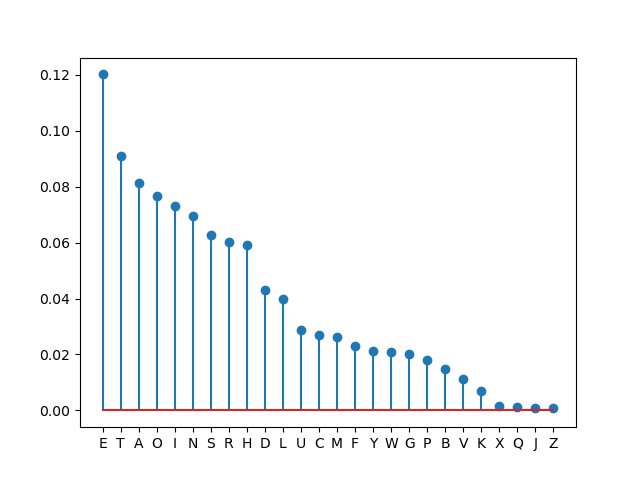
Fig. 1.7.1 Frequency Distribution of Letters in the English Language

We see that the entropy dropped to 4.18 indicating there is somewhat less disorder in a sequence of letters in an English text.

Shannon showed that the entropy of an ‘alphabet’ (the possible outcomes of our random variable) is the lower bound on the number of computer bits (0 or 1) needed to encode a typical (long) message. Indeed for a distribution for the English language we can do better then the 5 bits we classically need to encode 26 different letters.

The crux then is to use fewer bits for often occuring letters and use more bits for letters that occur less frequent. A nice example of such a coding scheme is the Morse alphabet. There every letter (and digit) is encodes with a sequence of ‘dots’ and ‘dashes’ (short and long tones). The international Morse codes are given in the table below

Fig. 1.7.2 Morse Codes (link to wikimedia.org)

Observe that indeed the number of dots and dashes are indeed roughly increasing with increasing frequency of the letter.

Unfortunately there is no constructive proof of Shannon’s result. Therefore there is no optimal algorithm for bit encoding. Perhaps the most famous one is Huffman encoding.

Without proof we give the Huffman encoding of the English alphabet:

Letter	Code	#bits	Letter	Code	n = #bits
E	011	3	M	00111	5
T	000	3	U	01001	5
A	1110	4	Y	00100	5
H	0101	4	B	101100	6
I	1100	4	G	111100	6
N	1010	4	P	101101	6
O	1101	4	V	001010	6
R	1000	4	W	111101	6
S	1001	4	K	0010111	7
C	01000	5	J	001011001	9
D	11111	5	Q	001011010	9
F	00110	5	X	001011011	9
L	10111	5	Z	001011000	9

Note that the number of bits is roughly inversely proportional to the probability of the letters. For a typical English text you would need on average

\[\sum_{x\in{A,\ldots,Z}} p(x) n(x) = 4.21 \,\text{bits}\]

a number that is rather close to the theoretical minimum of 4.18.

A bit allocation algorithm based on the frequencies of the different symbols, like Huffman encoding, is used in many compression schemes (e.g. JPEG image encoding).

1.7.3. Cross Entropy

Now consider the situation where we have a coding scheme (bit allocation) that is optimized for distribution \(q(x)\). However it turns out that in practice the true distribution is \(p(x)\). The expected number of bits per symbol then is:

\[H(p,q) = - \sum_{x} p(x) \log_2( q(x) )\]

This is called the cross entropy between distributions \(p\) and \(q\).

The cross entropy is often used in machine learning where we have a true a posteriori distribution \(p(x)\) over all class labels \(x\) and a distribution \(q(x)\) as predicted by our model. For binary logistic classification were \(p(x)\in\{y,1-y\}\) and \(p(q)\in\{\hat y, 1-\hat y\}\) where \(\hat y\) is the probability according to our model that \(x=1\). The cross entropy in that case is

\[H(p,q) = - y\log\hat y - (1-y)\log(1-\hat y)\]

This is the loss function (for one feature vector) as defined in logistic regression.

1.7.4. References

For a proper understanding of information theory and its use in Machine Learning and Coding/Compression we refer to

• Introduction to Data Compression by Khalid Sayood.

• Wikipedia (Entropy, Cross Entropy, Huffman)