1.3. Multivariate Functions

In programming we are accustomed to the fact that a function may take more then one argument to produce a result. For mathematical functions we also have functions with more then one argument: multivariate functions. As a simple example consider

\[f(x,y) = x^2+y.\]

Like we did for univariate functions we give a short overview of how to plot these multivariate functions, how to differentiate them and how to integrate them.

1.3.1. Plotting a multivariate function

Plotting multivariate functions in two arguments (we will call them 2D functions) is possible (given our capabilities of interpreting 2D drawings of 3D objects).

\[f(x,y) = x^2+y.\]

Show code for figure

import numpy as np
import matplotlib.pyplot as plt

x,y = np.meshgrid(np.linspace(-3, 3, 50), np.linspace(-3, 3, 50));
z = x**2 + y;
ax = plt.figure().add_subplot(projection='3d')
ax.plot_surface(x, y, z, linewidth=0,
                cmap=plt.cm.copper, rstride=1, cstride=1, shade=True);
plt.savefig('source/images/func2d.png')

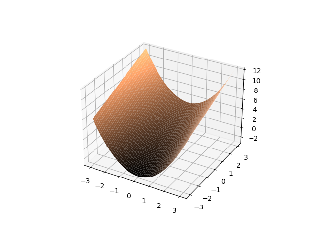
Fig. 1.3.1 Multivariate (2D) function plot.

klkll

Parameterized functions

For a fixed value \(y=a\) we may write \(f_a(x)=f(x,a)=x^2+a\) which you might recognize as a parameterized family of functions. For every value of \(a\) we have a new function. A 2D function can be viewed in a lot of ways as a parameterized family. We could fix \(x\) instead of \(y\). Doing this we see that for any \(a\) the function \(f(a,y)\) is a linear function in \(y\): \(f(a,y) = a^2+y\).

The shape of the function surface is easy to understand from the function recipe. For a \(y=0\) we have \(f(x,0)=x^2\) and as a function of \(x\) that is the parabola. For any value \(y=a\) we have a parabola in \(x\): \(f(x,a)=x^2+a\). For any value \(x=a\) we have straight line in \(y\): \(f(a,y)=a^2+y\). A 2D function in \(x\) and \(y\) thus can be seen as either a collection of 1D functions in \(x\) or a collection of functions in \(y\). In the figure below these collections of functions are embedded into the 3D space.

Show code for figure

xs = np.linspace(-3, 3, 50)
ys = np.linspace(-3, 3, 50)
N = len(xs)

fig = plt.figure(figsize=(8,4))
ax0 = fig.add_subplot(121, projection='3d')
ax1 = fig.add_subplot(122, projection='3d')

for y in ys[::4]:
    zs = xs**2 + np.full(N,y)
    ax0.plot(xs, np.full(N, y), zs)

for x in xs[::4]:
    zs = np.full(N, x**2) + ys
    ax1.plot(np.full(N, x), ys, zs)

plt.savefig('source/images/fxy_xy.png')

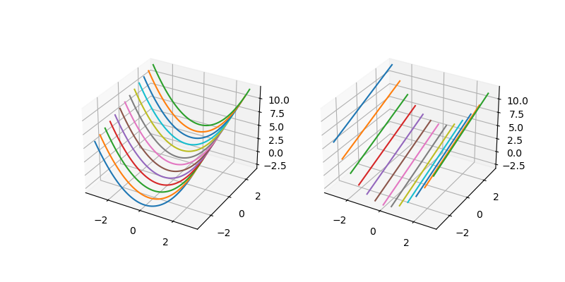
Fig. 1.3.2 Multivariate function plot. On the left we plot \(f(x,y)\) as a collection of 1D functions for several constant \(y\)-values. On the right we keep \(x\) constant.

Math doesn’t end with 1D or 2D functions. The simple extension is to add a time axis as well. Then images become video’s.

In many branches of computer science (statistical learning techniques for example) functions with hundreds, thousands and even millions of arguments are quite common. But our methods of visualizing multivariate functions do end with 2D functions (except when we add time). Beyond that, function (data) visualization involves some interpretation too, we have to select how to render the information in a 3D space that can be visualized. For that we refer to lectures on scientific visualization.

1.3.2. Differentiating a multivariate function

Continuity and Differentiability

A continuous 1D function is a function such that a very small change in the \(x\) value (say \(x+dx\)) leads to a very small change in the function value (\(f(x+dx)=f(x)+df\)). The notion of ‘’very small’’ can be given a rigerous definition in mathematics and we then refer to infinitesimals.

Note that not all continuous functions are differentiable. For instance the function \(|x|\) (the absolute value function) is not differentiable because for \(x=0\) the derivative is not uniquely defined. ‘Looking’ to the left from \(x=0\) the function has a slope \(-1\) and looking to the right the slope is \(+1\).

For more details see any textbook on calculus or look at Wikipedia for continuity and differentiability.

Remember the derivative of a univariate function:

\[\frac{df}{dx}(x) = \lim_{h\rightarrow0} \frac{f(x+h)-f(x)}{h}\]

So the derivative measures something like the rate of change. It gives the change in value when we change the argument a little bit. Derivatives are therefore the mathematical way of describing change. For a univariate function the derivative at \(x=a\) is the slope of the tangent line to the function in \((a,f(a))\).

The derivative of a function \(f\) is also a function. Taking the derivative thus transforms a function into a new function. The derivative function is often denoted as \(f'\).

We can take the derivative of the derivative. Then we calculate the change in the slope as we move a little along the horizontal axis. The second derivative is denoted as \(f''=\frac{d^2f}{dx^2}\). In the same way we can calculate the derivative up to any order (3th, 4th etc).

Differentiating a multivariate function is somewhat more complex. The idea is the same: what happens to the function value when I change the input just a little? But what do I mean now with changing the input? Should all the arguments be changed, or just one? Well actually it is your choice, there is a need for both these options in practice.

A Note on Notation

Given a function \(f(x,y)\) its partial derivative up to order 2 are:

\[\begin{split}f_x = \partial_x f = \pfrac{f}{x}\\ f_y = \partial_y f = \pfrac{f}{y}\\ f_{xx} = \partial_{xx} f = \pfrac{^2 f}{x^2}\\ f_{xy} = \partial_{xy} f = \pfrac{^2 f}{xy}\\ f_{yy} = \partial_{yy} f = \pfrac{^2 f}{y^2}\end{split}\]

Note that all derivatives of \(f\) are 2D multivariate functions. E.g. the value \(f_y\) at \((x,y)\) is written as \(f_y(x,y) = \partial_y f(x,y) = \pfrac{f(x,y)}{y}\) or also as \(\pfrac{f}{y}(x,y)\). There is no strict rule on this in machine lecture literature.

The simplest one is to change only one of the arguments and see what happens to the function value. Consider the function \(f\) in two arguments, say \(x\) and \(y\). Let us change \(x\) to \(x+h\), while keeping \(y\) fixed! We could then calculate what is known as the partial derivative of \(f\) with respect to its first argument which is called \(x\).

\[\frac{\partial}{\partial x} f(x,y) = \lim_{h\rightarrow0} \frac{f(x+h,y)-f(x,y)}{h}\]

Observe that instead of \(df/dx\) we write \(\partial f/\partial x\) to distinguish between the derivative of a univariate function and the derivative with respect to just one argument (the one that by convention is called \(x\)) of a multivariate function. Be sure to understand that the partial derivative of a multivariate function results in a multivariate function in the same number of arguments.

The partial derivative in the \(y\) argument is:

\[\frac{\partial}{\partial y} f(x,y) = \lim_{h\rightarrow0} \frac{f(x,y+h)-f(x,y)}{h}\]

At high school you have learned how to calculate the derivatives of functions. Better said you were given the derivatives of some basic functions (like \(x^n\), \(\cos(x)\), \(\log(x)\) and others) and the rules to calculate the derivatives of compound functions (like the chain rule and the product rule). Can we use this knowledge for partial differentiation as well? Yes we can. Remember when we are (partially) differentiating \(f\) with respect to \(x\) we keep \(y\) fixed and thus while differentiating anything in the formula with a \(y\) in it, it is treated as a constant.

For instance consider \(f(x,y)=x^2+y\). Differentiating with respect to \(x\) leads to \(2x\). The rules to follow here are:

• the derivative of a sum is the sum of the derivatives, so we may take the derivative of \(x^2\) plus the derivative of \(y\).

• the derivative of \(x^2\) with respect to \(x\) is equal to \(2x\)

• the derivative of \(y\) with respect to \(x\) is \(0\).

The partial derivative with respect to \(y\) is a constant function equal to \(1\) everywhere (note that the term \(x^2\) now is taken to be fixed, i.e. constant with zero derivative). So let

\[f(x,y) = x^2 + y,\]

then we have:

\[\begin{split}\pfrac{f}{x} (x,y) &= 2x\\ \pfrac{f}{y} (x,y) &= 1.\end{split}\]

A bit more complex example. Let

\[f(x,y) = x\cos(a x + by) + y\sin(a x + by)\]

then:

\[\begin{split}\pfrac{f}{x} (x,y) &= \cos(a x + by) - a x \sin(a x + b y) + a y \cos(a x + by)\\ &= (1+ay)\cos(a x + b y) - a x \sin(ax + by)\end{split}\]

Also for partial derivatives we may repeat the differentiation. So the second order derivative in the \(x\) argument is denoted as \(\partial^2 f / \partial x^2\). But now we can do something else as well: first take the derivative in \(x\) direction followed by taking the derivative in \(y\) direction. Or the other way around: first \(y\) then \(x\). It can be shown that for all ``nice’’ functions (``nice’’ meaning that these two derivatives are continuous) the order in which the derivatives are taken does not matter. We have:

\[\frac{\partial^2 f}{\partial x \partial y} = \frac{\partial^2 f}{\partial y \partial x}\]

The partial derivatives play an important role in the analysis of local structure in images. To make notation a bit simpler there we will use the subscript notation for partial derivatives. Let \(f\) be a 2D function with arguments we name \(x\) and \(y\). The partial derivative with respect to \(x\) is denoted as \(f_x\), and the second partial derivative both with respect to \(x\) as \(f_{xx}\). The mixed second order derivative if \(f_{xy}\).

The order of differentiation of a multivariate function is the total number of times we do a differentiation, no matter in which argument. So \(f_x\) and \(f_y\) are first order derivatives, whereas \(f_{xx}\), \(f_{xy}\) and \(f_{yy}\) are second order derivatives. Note that \(f_{xxy}\) is a third order derivative.

1.3.3. Properties of Differentiation

Most of the properties are direct generalizations of the properties we have seen for univariate functions:

• The derivative (any of the partial derivatives) distributes over a sum of functions, i.e. the derivative of a sum is the sum of the derivatives.

• The product rule behaves just like it did for univariate functions, although the results become rapidly messy in case you are looking at higher order mixed derivatives (like \(\partial_{xxxyy}\).

• The chain rule of differentiation requires some careful thought:

Consider the function \(g(x,y) = f(u(x,y), v(x,y))\) and we want to calculate the partial derivative \(\partial_x g(x,y)\). To simplify notation we observe that \(f\) is dependent on \(u\) and \(v\) and that both \(u\) and \(v\) are dependent on \(x\) and \(y\). Keeping this in mind we will often omit the arguments of the functions involved.

Theorem 1.3.1 (Multivariate Chain Rule)

Let \(g(x,y) = f(u(x,y), v(x,y))\) where all functions \(g\), \(f\), \(u\) and \(v\) are functions in two arguments. The multivariate chain rule then states that:

\[\partial_x g(x,y) = \partial_u f(u(x,y), v(x,y)) \partial_x u(x,y) + \partial_v f(u(x,y),v(x,y)) \partial_x v(x,y)\]

showing that we apply the univariate chain rule for both arguments \(u\) and \(v\) and add the contributions. Using the \(g_x\) notation to indicate the derivative \(\partial_x g\) and omitting all \(x,y\) arguments for \(f\), \(u\) and \(v\) and also leaving out the arguments \(u,v\) for \(f\) the above can be written as:

\[g_x = f_u u_x + f_v v_x\]

or equivalently:

\[\pfrac{g}{x} = \pfrac{f}{u}\pfrac{u}{x} + \pfrac{f}{v}\pfrac{v}{x}\]

Proof

As often we start with the definition:

\[\begin{split}g_x(x,y) &= \lim_{h\rightarrow0}\left( \frac{g(x+h)-g(x)}{h} \right)\\ &=\lim_{h\rightarrow0}\left( \frac{f(u(x+h,y), v(x+h,y)) - f(u(x,y), v(x,y)))}{h} \right)\end{split}\]

Now consider the term \(u(x+h,y)\). For \(h\rightarrow0\) we allready know we can write this as \(u(x,y) + h u_x(x,y)\). Using the equivalent expression for \(v(x+h,y)\) the above equation turns into:

\[\begin{split}g_x(x,y) &= \lim_{h\rightarrow0}\left( \frac{f(u(x,y) + h u_x(x,y), v(x,y) + h v_x(x,y)) - f(u(x,y), v(x,y)))}{h} \right)\\\end{split}\]

Omitting the \(x,y\) arguments we have:

(1.3.1)\[\begin{split}g_x &= \lim_{h\rightarrow0}\left( \frac{f(u + h u_x, v + h v_x) - f(u, v))}{h} \right)\\\end{split}\]

Now we can apply the same ‘trick’ to \(f\), but now we have ‘\(h\)-terms’ in both arguments of \(f\). We start with the first argument:

\[f(u + h u_x, v + h v_x) = f(u, v + h v_x) + h f_u(u, v + h v_x) u_x\]

and then for the second argument of \(f\) and \(f_u\):

\[\begin{split}f(u + h u_x, v + h v_x) &= f(u,v) + h f_v(u,v) v_x + h \left( f_{u}(u,v) + h f_{uv} u_x \right) \\ &= f(u,v) + h f_v(u,v) v_x + h f_{u}(u,v) + h^2 f_{uv} u_x\end{split}\]

Substituting this into Eq.1.3.1 we get

\[\begin{split}g_x &= \lim_{h\rightarrow0}\left( \frac{f(u,v) + h f_v(u,v) v_x + h f_{u}(u,v) + h^2 f_{uv} u_x- f(u, v))}{h} \right)\\ &= \lim_{h\rightarrow0}\left( f_v(u,v) v_x + f_{u}(u,v) + h f_{uv} u_x\right)\\ &= f_v(u,v) v_x + f_{u}(u,v)\end{split}\]

1.3.4. Integration of Multivariate Functions

Fig. 1.3.3 A 2D function and the integral of \(f(x,y)\) over the rectangular domain at the bottom is the volume under the graph of the function.

Consider the multivariate function:

\[f(x,y) = 10 - \frac{x^2-y^2}{8}\]

with a plot shown in the figure to the right. The integral

\[V = \iint_R f(x,y)dx dy\]

calculates the volume under the graph of the function.

We need not stop with functions in two arguments. Consider the function \(f\) in \(n\) arguments

\[f(x_1,\ldots,x_n).\]

For \(n>2\) we cannot draw the function surface anymore but a lot of the intuition from lower dimensional functions is applicable. Also for integration. Again we can calculate the hypervolume underneath the graph of the function

\[V = \iint\cdots\iint_A f(x_1,\ldots,x_n) dx_1\cdots dx_n\]

Fig. 1.3.4 Riemann sum for a 2D function \(f(x,y)\).

Observe that we can set up a Riemann limit definition in this case as well. Now \(dx dy\) is the area of an infinitesimal part of the rectangular domain and \(f(x,y)\) is the height. So \(f(x,y)dx dy\) is the volume under the graph of \(f(x,y)\) above that infinitesimal area.

Analytical calculation of multivariate integrals can become quite complex, especially when the domain of integration is not axis aligned (for instance if we want to know the volume under the function in the domain \(x^2+y^2<1\)).

In this introductory course we (fortunately) do not need to analytically calculate these integrals and we leave that subject to another course (and Mathematica and mathematicians…).

1.3.5. Symbolic Math Computations

Computer scientists are (in most cases) no mathematicians. So doing a lot of tedious, error prone math (be it calculus, linear algebra or any other branch) is not our joy in life. Fortunately there are symbolic math programs to solve most of our day to day needs.

There are many great programs for symbolic math. Mathematica is perhaps the best known. Mathematicians themselves tend to use Maple more in my perception. Other symbolic math programs do exist.

Here we will use SymPy that is an extension for Python to deal with some simple symbolic math.

from sympy import Symbol, diff, exp, simplify, init_printing, latex

init_printing()
x = Symbol("x"); y = Symbol("y"); a = Symbol("a");
f = x**2+y
print(f)
print(diff(f, x))
print(diff(f, y))
print(diff(f, x, 2))
f = exp(-a*(x**2+y**2));
print(f)
print(diff(f,x,1))
print(diff(f,y,1))
print(simplify(diff(f,x,2)))
print(simplify(diff(f,x,1,y,1)))
print(simplify(diff(f,y,2)))

x**2 + y
2*x
1
2
exp(-a*(x**2 + y**2))
-2*a*x*exp(-a*(x**2 + y**2))
-2*a*y*exp(-a*(x**2 + y**2))
2*a*(2*a*x**2 - 1)*exp(-a*(x**2 + y**2))
4*a**2*x*y*exp(-a*(x**2 + y**2))
2*a*(2*a*y**2 - 1)*exp(-a*(x**2 + y**2))

1.3.6. Exercises

1. In a previous section we have looked at the function

   \[f(x,y) = x\cos(a x + by) + y\sin(a x + by)\]

   and given its first order partial derivative with respect to \(x\), i.e. \(\partial_x f\).

   Also calculate \(\partial_y f\), \(\partial_{xx} f\), \(\partial_{xy} f\) and \(\partial_{yy} f\)

2. Calculate all partial derivatives up to order 2 of the functions:

   \[\begin{split}f(x,y) &= \exp\left( - a(x^2+y^2) \right)\\ g(x,y) &= \cos(a x + b y)\end{split}\]

   i.e. calculate \(f_x=\partial_x f\), \(f_y\), \(f_{xx}\), \(f_{xy}\) and \(f_{yy}\) and the same derivatives but then for the function \(g\).

3. Given:

   \[g(x,y,s) = \frac{1}{2\pi s^2}\exp\left( -\frac{x^2+y^2}{2s^2} \right)\]

   calculate \(g_s = \partial_s g = \frac{\partial g}{\partial s}\).