\(\newcommand{\prt}{\partial}\) \(\newcommand{\pfrac}[2]{\frac{\prt #1}{\prt #2}}\)

1.6. Computational Graphs and the Chain Rule of Differentiation

We start by introducing computational graphs as a simple visualization of the flow of data within a typical machine learning system (neural networks as prime examples) by defining the sequence(s) of computations necessary to calculate the end result.

The final step in a computational graph (when learning) is the calculation of the loss that quantifies the error that the system makes when processing the input data.

These computational graphs not only describe the ‘forward’ flow of the data (from input data to output) but

In order to understand automatic differentiation we first have to look at computational graphs. Then using these graphs we look at automatic differentiation.

1.6.1. Computational Graph

A computational graph describes the ‘flow of data’ throughout a computation. Consider the expression \(z=log(3x^2 + 5 xy)\) in a graph this can be depicted as:

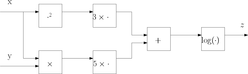
Fig. 1.6.1 Computational Graph for the expression \(z=log(3x^2 + 5 xy)\)

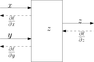
Fig. 1.6.2 Computational graph with backward differentaion arrows for the expression \(z=z(x,y)\)

1.6.2. Automatic Differentiation

We are going to use automatic differentiation to calculate \(\prt z/\prt x\) and \(\prt z/\prt y\). To start we look at one node representing the expression

\[z = z(x,y)\]

and imagine that this node is part of a larger graph ending up in the final scalar value \(\ell\). Now assume that somehow we were capable of calculating \(\prt \ell/\prt z\). What then are the derivatives \(\prt\ell/\prt x\) and \(\prt\ell/\prt y\)?

For the derivative with respect to \(x\) we have:

\[\pfrac{}{x} \ell(z(x,y)) = \pfrac{\ell}{z} \pfrac{z}{x}\]

and for the derivative with respect to \(y\):

\[\pfrac{}{y} \ell(z(x,y)) = \pfrac{\ell}{z} \pfrac{z}{y}\]

It should be noted that the notation \(\ell(z(x,y))\) is a bit misleading. It is just to illustrate that \(\ell\) depends on \(z\), in a complex graph it will probably depend on many other values.

The important observation is that for any node in the graph, given the derivative of the output \(\ell\) of the entire graph with respect to the output of this one node, we can calculate the derivative of \(\ell\) with respect to the inputs of this node. If that is true, then we are able to ‘propagate’ the derivative calculations from the end of the graph ‘backwards’ to the beginning. This is essentially what backpropagation does in neural network learning.

1.6.3. Example

Let’s do it for our first example:

\[z = \log(3 x^2 + 5 x y)\]

Using the chain rule and some basic derivative rules we have:

\[\begin{split}\pfrac{z}{x} &= \frac{6x+5y}{3x^2+5xy}\\ \pfrac{z}{y} &= \frac{5x}{3x^2+5xy}\\\end{split}\]

where we have assumed that \(\log\) is the natural logarithm (as most programming languages do as well). Let’s see whether we can reproduce these results using the computational graph. First we redraw the graph and name all arrows (values) in the graph for ease of reference.

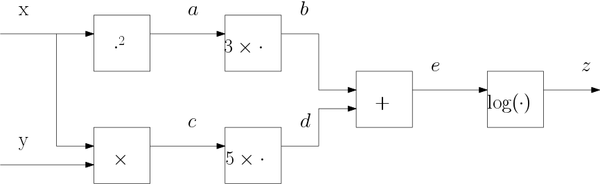
So we have:

\[\begin{split}a &= x^2\\ b &= 3 a\\ c &= x y\\ d &= 5 c\\ e &= b +d\\ z &= \log(e)\end{split}\]

and no, \(e\) is not the Working from the end to the start we get

\[\begin{split}\pfrac{z}{e} &= \frac{1}{e}\\ \pfrac{z}{b} &= \pfrac{z}{e}\\ \pfrac{z}{d} &= \pfrac{z}{e}\\ \pfrac{z}{a} &= \pfrac{z}{b} 3\\ \pfrac{z}{c} &= \pfrac{z}{d} 5\\ \pfrac{z}{y} &= \pfrac{z}{c} x\end{split}\]

The above steps are easy, but what about the derivative of \(z\) with respect to \(x\). There we see that the value of \(x\) is fed into two nodes in the graph. So from the two ‘streams’ starting at \(x\) when considering the backward pass we see to derivatives

\[\pfrac{a}{x} \pfrac{z}{a}\quad \text{and}\quad \pfrac{c}{x} \pfrac{z}{c}\]

to calculate \(\prt z/\prt z\) we have to add these contributions:

\[\begin{split}\frac{z}{x} &= \pfrac{a}{x} \pfrac{z}{a} + \pfrac{c}{x} \pfrac{z}{c}\\ &= 2x \pfrac{z}{a} + y \pfrac{z}{c}\end{split}\]

This leads to

\[\begin{split}\pfrac{z}{x} &= 2x \pfrac{z}{a} + y \pfrac{z}{c}\\ &= \frac{6x}{3x^2+5 xy} + \frac{5y}{3x^2+5xy} &= \frac{6x+5y}{3x^2+5 xy}\end{split}\]

The derivation of \(\prt z/\prt y\) is left to the reader as an exercise.

1.6.4. Numerical Example

Computational graphs and automatic differentiation can be used to derive formula’s but that is not the way they are used in practice. In practice they are used to calculate the derivatives numerically for a given set of inputs. Consider again our example graph but now with input \(x=2\) and \(y=3\).

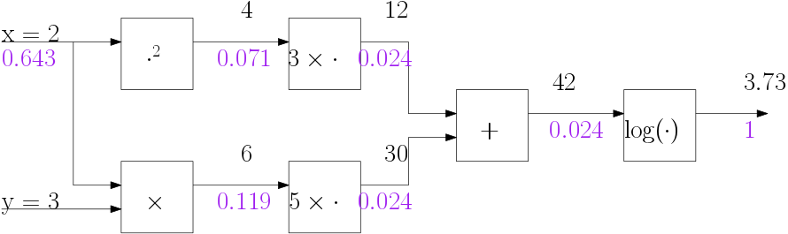
Calculating the intermediate values then constitutes the forward pass:

\[\begin{split}a = 4\\ b = 12\\ c = 6\\ d = 30\\ e = 42\\ z = \log(42) = 3.73\end{split}\]

The backward pass numerically is simple and we have indicated the values below the edges in the graph above. Be sure to understand how the purple values are calculated.

1.6.5. Vectorial Graphs

In neural networks the nodes in graphs take vectorial input and produce vectorial output. Consider the node that takes \(\v x\in\setR^n\) as input and produces \(\v y\in\setR^m\) as output. In formula:

\[\v y = \v f(\v x)\]

and in a graph:

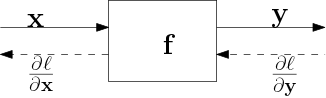
Fig. 1.6.3 Vectorial Function Node

Note that \(\v f\) is a function that takes a vector and produces a vector. In element notation we have:

\[\begin{split}\begin{pmatrix}y_1\\\vdots\\y_m\end{pmatrix} = \begin{pmatrix} f_1(x_1,\ldots,x_n)\\ \vdots\\ f_m(x_1,\ldots,x_n) \end{pmatrix}\end{split}\]

Note that we may write \(\ell(y_1,\ldots,y_m)\) to indicate the \(\ell\) is dependent on all components of \(\v y\). Note that eacht \(y_j\) is dependent on all \(x_i\), i.e. \(y_j = f_j(x_1,\ldots,x_n)\). Constructing \(\prt \ell/\prt \v x\) elementwise we have:

\[\pfrac{\ell}{x_i} = \pfrac{\ell(y_1,\ldots,y_m)}{x_i} = \sum_{j=1}^{m} \pfrac{\ell}{y_j} \pfrac{f_j}{x_i}\]

We define the matrix \(J\) such that

\[J_{ij} = \pfrac{y_j}{x_i}\]

then:

\[\pfrac{\ell}{x_i} = \sum_{j=1}^{m} J_{ij} \pfrac{\ell}{y_j}\]

as vectors we can write:

\[\pfrac{\ell}{\v x} = J \pfrac{\ell}{\v y}\]

The matrix \(J\) is called the Jacobian of the function \(\v f\) and is often denotes as

\[J = \pfrac{\v f}{\v x}\]

When using vectorial graphs in neural networks we will see that the Jacobian matrices are often of a special form due to the choice of the function \(\v f\).

1.6.6. PyTorch

There are many libraries that use automatic differentiation in computational graphs for machine learning purposes, here we look at PyTorch only.

Consider the calculation that served as our example in this section:

\[z = 3x^2+5xy\]

In Pytorch we can write

In [1]: import torch

In [2]: x = torch.tensor([2.0], requires_grad=True)

In [3]: y = torch.tensor([3.0], requires_grad=True)

In [4]: z = torch.log(3*x**2 + 5*x*y)

In [5]: print("z = ", z)
z =  tensor([3.7377], grad_fn=<LogBackward0>)

In [6]: z.backward()

In [7]: print("x.grad = ", x.grad)
x.grad =  tensor([0.6429])

In [8]: print("y.grad = ", y.grad)
y.grad =  tensor([0.2381])

In torch the tensors take the place of the ndarrays from numpy. Special in torch is that the ‘requires_grad=True’ flag ensures that any expression involving tensors with that attribute are differentiable with respect to these tensors. Convince yourself that ‘x.grad’ is indeed the value of \(\prt\ell/\prt x\) as defined and calculated in a previous section.

The ‘magic’ of PyTorch Autograd functionality is that we don’t need to build the graph explicitly as in Tensorflow. By using ‘requires_grad=True’ in the leaf nodes of the graph the call to ‘backward()’ on a node in the calculation depending on those leave nodes leads to the calculation of the derivatives of the final value (where ‘backward()’ was called with respect to the leave node values.

We can calculate all intermediate value is the backward propagation but then we have to explicitly encode all intermediate steps and make sure these steps remember (retain) their derivative values.

In [9]: x = torch.tensor([2.0], requires_grad=True)

In [10]: y = torch.tensor([3.0], requires_grad=True)

In [11]: a = x**2; a.retain_grad()

In [12]: b = 3 * a; b.retain_grad()

In [13]: c = x * y; c.retain_grad()

In [14]: d = 5 * c; d.retain_grad()

In [15]: e = b + d; e.retain_grad()

In [16]: z = torch.log(e); z.retain_grad()

In [17]: z.backward(retain_graph=False)

In [18]: print(z)
tensor([3.7377], grad_fn=<LogBackward0>)

In [19]: print("x grad = ", x.grad)
x grad =  tensor([0.6429])

In [20]: print("y grad = ", y.grad)
y grad =  tensor([0.2381])

In [21]: print("a grad = ", a.grad)
a grad =  tensor([0.0714])

In [22]: print("b grad = ", b.grad)
b grad =  tensor([0.0238])

In [23]: print("c grad = ", c.grad)
c grad =  tensor([0.1190])

In [24]: print("d grad = ", d.grad)
d grad =  tensor([0.0238])

In [25]: print("e grad = ", e.grad)
e grad =  tensor([0.0238])

In [26]: print("z grad = ", z.grad)
z grad =  tensor([1.])

This section is certainly not a guide of how to use the Pytorch Autograd module. It merely shows what the library is capable of.