1.2. Univariate Functions

1.2.1. Definition

A univariate function is what you have learned in high school. A univariate function \(f\) takes one input number, say \(x\), and produces one output number \(y\). We write

\[y = f(x)\]

The value \(x\) is called the argument of the function. And just like in programming the naming of the argument is irrelevant. For instance if we define the function \(f(x)=x^3\) using

def f(x):
    return x * x * x

we may call it with

a = 2
print(f(a))

The function happily accepts its one argument value (in this case equal to 2) and calculates the result. So the function itself is unaware of what name you have for the argument. [1]

On the other hand the function also is not dependent on what name for the argument you have chosen in the function definition, solid

def f(a):
    return a * a * a

really is the same function! We will return to this delicate interplay between arguments and their naming convention in the section on multivariate functions..

Let’s define a function with

\[f(x) = \sin(x) + 0.2 \sin(3x)\]

In Python we can define and plot the function quite easily:

import numpy as np
import matplotlib.pyplot as plt


plt.clf()

def f(x):
    return np.sin(x) + 0.2 * np.sin(5*x) + 2

x = np.linspace(0, 3*np.pi, 1000)
plt.plot(x, f(x), label=f"$f(x)$")
plt.legend()
plt.savefig('source/images/univariateplot.png')

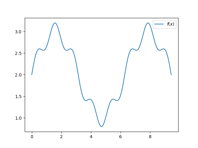
Fig. 1.2.1 Univariate function plot.

Observe that the Python matplotlib plot function is given x and f(x) as arguments where x is an array of 1000 real values in the interval from \(0\) to \(3\pi\) and f(x) also is a 1000 element array with all function values.

The values of \(f(x)\) that falls in between two of the sample points are not calculated and matplotlib simply draws a straight line (play with the number of points in the linspace function call.

1.2.2. Differentiating Univariate Functions

In machine learning, differentiation is everywhere. So to refresh your memory on this we will look at the definition, the derivatives of some basic function and the properties that allows us to calculate the derivative of (nearly) every function.

Definition 1.2.1 (Differentiating)

Let \(f(x)\) be a function \(f: \setR\rightarrow\setR\), i.e. a function that takes a real number as argument and returns a real number, then its derivative \(f'\) is also \(f': \setR\rightarrow \setR\) and is defined as:

\[f'(x) = \lim_{h\rightarrow0} \frac{f(x+h)-f(x)}{h}\]

The geometrical interpretation of the derivative is that \(f'(x)\) is the slope of the tangent line to the graph of the function in point \(x\) as illustrated in Fig. 1.2.2,

Show code for figure

plt.clf()
x = np.linspace(3/2*np.pi, 2*np.pi, 1000)
x0 = 5.3
fx0 = f(x0)
plt.plot(x, f(x), linewidth=3, label=f"$f(x)$")
plt.scatter([x0], [f(x0)])
plt.stem([x0], [fx0])
plt.axhline(0)
plt.text(x0-0.02, -0.1, f"$x_0$")

def fp(x):
    return np.cos(x) + np.cos(5*x)

def tangentf(x0, x):
    fx0 = f(x0)
    fpx0 = fp(x0)
    return fpx0 * x + fx0 - fpx0 * x0

plt.plot(x, tangentf(x0, x), label='tangent line')

x5 = 5
x6 = 6
fx5 = f(x5)
fx6 = f(x6)
plt.plot([x5, x6, x6], [tangentf(x0, x5),
   tangentf(x0, x5), tangentf(x0, x6)])

plt.text(5.5, fx5+0.05, "1")
plt.text(6, 1.4, f"$f'(x_0)$")
plt.legend()
plt.savefig('source/images/oneDderivative.png')

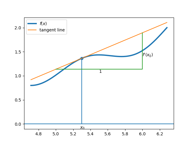
Fig. 1.2.2 The derivative \(f'(x)\) is the slope of the tangent line in point \(x\).

In this course we most often assume that a function \(f\) has a unique and well defined derivative \(f'(x)\) for every \(x\) in its domain. An exception to this rule is the ReLU function defined with:

\[f(x) = \max(0, x)\]

that has a derivative for all \(x\) except for \(x=0\) where its derivative is not defined. [2] Such a function is called almost everywhere differentiable, a term that is given a formal definition in math (but we won’t look into that in this course).

The operator that differentiates a function is denoted as:

\[\frac{d}{dx}\]

so

\[f' =\frac{df}{dx}\]

Here you should read \(dx\) as refering to denominator \(h\) in definition 1.2.1, the infinitesimal deviation of the variable \(x\). Then \(df\) refers to the numerator \(f(x+h) - f(x)\), the infinitesimal deviation of \(f\) at \(x\). You will often see computer scientists write \(dx\) instead of a variable \(h\) together with an explicit limit \(\lim_{h \to 0}\) for this reason.

Observe that the derivative \(f'\) is a function as well and we can take the derivative of that as well:

\[f'' =\frac{df'}{dx} = \frac{d}{dx}\frac{df}{dx} = \frac{d^2f}{dx^2}\]

And we can keep going on looking at the \(n\)-th order derivative of a function.

There are a lot of different notational conventions to denote the derivative. Let \(y=f(x)\) then we have

\[\frac{d}{dx} f = y' = \frac{dy}{dx} = f'(x) = \frac{df(x)}{dx} = d_x f(x)\]

1.2.2.1. Derivatives of Standard Functions

The derivatives of the following standard functions are used in this machine learning course.

Table 1.2.1 Derivatives of Standard Functions

\(f(x)\)	\(f'(x)\)
c	0
\(x^n\)	\(n x^{n-1}\)
\(\sin(x)\)	\(\cos(x)\)
\(\cos(x)\)	\(-\sin(x)\)
\(e^x\)	\(e^x\)
\(\ln(x)\)	\(\frac{1}{x}\)

The derivatives in the table are all provable using the limit definition of differentiation. Let’s consider a simple one: the derivative of the sine function.

Theorem 1.2.2 (The derivative of the sine function is the cosine function:)

\[\frac{d}{dx} \sin(x) = \cos(x)\]

Proof (well… not really a proof)

By definition we have:

\[\frac{d}{dx} \sin(x) = \lim_{h\rightarrow0} \frac{\sin(x+h) - \sin(x)}{h}\]

Remember this from highschool: \(\sin(x+y) = \sin(x)\cos(y) + \cos(x)\sin(y)\). Using this in the above we get:

\[\frac{d}{dx} \sin(x) = \lim_{h\rightarrow0} \frac{\sin(x)\cos(h) + \cos(x)\sin(h) - \sin(x)}{h}\]

Note that for \(h\rightarrow0\) we have that \(\cos(h)\rightarrow1\) and \(\sin(h)\rightarrow h\) and thus:

\[\frac{d}{dx} \sin(x) = \lim_{h\rightarrow0} \frac{ \cos(x) h}{h} = \cos(x)\]

which ‘proves’ our theorem [3]

Theorem 1.2.3 (Derivative of the power function \(x^n\))

The derivative of the power function \(x^n\), for any real valued \(n\), is given by:

\[\frac{d}{dx} x^n = n x^{n-1}\]

Proof

Again the proof is not too difficult, i.e. when considering \(n\in \mathbb N\). But it can also be shown that even for negative integers this rule is true. And it is even true for all fractional valued \(n\).

1.2.2.2. Rules for Derivatives

If a more complex function is composed out of the basic functions like \(\sin(x^2)\) or \(\sin(a x) + b\cos(5x)\) we can use the differentiation rules to calculate its derivative:

Theorem 1.2.4 (Multiplication with a constant)

\[\frac{d}{dx} c f(x) = c \frac{d}{dx} f(x) = c f'(x)\]

Proof

This proof is actually really simple. Just use the limit definition of the derivative while noting that the constant can be taken out of the limit.

Theorem 1.2.5 (Sum rule)

The derivative of the weighted sum of functions is equal to the weighted sum of the derivatives of those functions. Let \(f\) and \(g\) be two functions with derivatives \(f'\) and \(g'\) and let \(a\) and \(b\) be two real values, then:

\[\frac{d}{dx}\left( a f(x) + b g(x)\right) = a f'(z) + b g'(x)\]

Proof

Again the proof is simple using the limit definition when observing that the limit of a sum of functions is equal to the sum of the limits of those functions.

Theorem 1.2.6 (Product Rule)

Let \(f\) and \(g\) be two functions with derivatives \(f'\) and \(g'\) then:

\[\frac{d}{dx} f(x)g(x) = f'(x)g(x) + f(x)g'(x)\]

Proof

This proof is a bit more tricky and is based on a familiar ‘trick’ of adding \(0\). In this case we add zero to the numerator in the limit definition.

By definition we have:

\[\frac{d}{dx} f(x)g(x) = \lim_{h \rightarrow0} \frac{f(x+h)g(x+h) - f(x)g(x)}{h}\]

Now we add \(0 = f(x+h)g(x) - f(x+h)g(x)\) to the numerator:

\[\begin{split}\frac{d}{dx} f(x)g(x) &= \lim_{h \rightarrow0} \frac{f(x+h)g(x+h) - f(x+h)g(x) + f(x+h)g(x) - f(x)g(x)}{h}\\ &= \lim_{h\rightarrow0} f(x+h) \frac{g(x+h)-g(x)}{h} + \lim_{h\rightarrow0} g(x) \frac{f(x+h)-f(x)}{h}\end{split}\]

where in the last step we, again, have used the fact that the limit of a sum is the sum of the limits (if both limits exist). In the same way the limit of a product of functions is the product of the limits of those functions. Note that the limit for \(h\rightarrow0\) of \(f(x+h)\) equals \(f(x)\). This leads to

\[\begin{split}\frac{d}{dx} f(x)g(x) &= f(x) \lim_{h\rightarrow0} \frac{g(x+h)-g(x)}{h} + g(x) \lim_{h\rightarrow0} \frac{f(x+h)-f(x)}{h}\\ &= f(x)g'(x) + g(x)f'(x) = f'(x)g(x) + f(x)g'(x)\end{split}\]

Besides the product rule we also have the quotient rule.

Theorem 1.2.7 (Quotient Rule)

Let \(f\) and \(g\) be two functions with derivatives \(f'\) and \(g'\), then:

\[\frac{d}{dx} \frac{f(x)}{g(x)} = \frac{f'(x) g(x) - f(x)g'(x)}{g^2(x)}\]

Proof

The proof simply follows from the product rule writing \(f(x)/g(x) = f(x)(g(x))^{-1}\) and using the chain rule. The proof is left as an exercise to the reader.

And finally the property that is of enormous importance in machine learning: the chain rule for differentiation.

Theorem 1.2.8 (The Chain Rule)

Let \(h(x) = g(f(x))\) then

\[h'(x) = g'(f(x)) f'(x)\]

Proof (The Chain Rule)

For infinitesimal \(dx\), i.e. \(dx\to 0\), we have

\[h(x+dx) = h(x) + h'(x) dx\]

Now we do the same for \(h(x)=g(f(x))\):

\[\begin{split}h(x+dx) &= g(f(x+dx))\\ &= g(f(x)+f'(x)dx)\\ &= g(f(x)) + g'(f(x))f'(x)dx\\ &= h(x) + g'(f(x)) f'(x) dx\end{split}\]

Comparing both expressions for \(h(x+dx)\) we get:

\[h'(x) = g'(f(x)) f'(x)\]

The chain rule is so important in machine learning that a special section in these lecture notes is devoted to it.

1.2.3. Integrating Univariate Functions

Integral = Area under Curve

In probability theory and thus in machine learning we need integration of functions besides differentiation. Consider the function \(f\). Then we think of the integral

\[\int_{a}^{b} f(x) dx\]

to stand for the area under the curve of \(f\), i.e. for each \(x\) we consider all between \(0\) and \(f(x)\). If \(f(x)<0\) then the contribution is counted negatively. As an example consider the integral from \(0\) to \(2\pi\) of the sine function. From \(0\) to \(\pi\) the contribution is positive, but from \(\pi\) to \(2\pi\) the contribution is negative and the total integral is \(0\).

Riemann Integral

Just like differentiation can be defined as a limit of the differential quotient, the integral can also be described as a limit. First the interval from \(a\) to \(b\) on the x-axis is subdivided into \(n\) intervals of width \(dx\). The subintervals then are

\[[x_i, x_{i+1}] = [i\, dx, (i+1)\,dx]\]

Consider one of these intervals from \(x_i\) to \(x_{i+1}\), then we approximate the area under the curve in this subinterval as the width times the height of the rectangular bar of width and height \(f(x_i)\). The approximated integral then is the sum of all areas associated with all subintervals in the interval \([a,b]\). The integral then is the limit when letting \(n\rightarrow\infty\) (or \(dx\rightarrow0\)):[4]

\[\int_a^b f(x)dx = \lim_{n\rightarrow\infty} \sum_{i=0}^{n-1} f(x_i) dx\]

Having an intuition that an integral calculates the area under a curve does not give us a nice way of calculating an integral. The fundamental theorem of calculus links integrals and derivatives.

Theorem 1.2.9 (Fundamental Theorem of Calculus)

Let \(F\) be a function with derivative \(f\), i.e.

\[\frac{d}{dx} F = F' = f\]

then

\[\int_a^b f(x) dx = F(b)-F(a)\]

Proof (FTC)

If you want to take a look at the proof read this. The proof is not part of the course. But it is nice to observe that you should be able to follow that proof.

The FTC in a way is the `inverse’ of what we want in practice. Then the function \(f\) is given (the integrand in this case). Let we assume that \(F'=f\) so \(F\) is the function we need to calculate the integral of. But if \(F'=f\) then also \((F+c)' = f\) for any scalar constant \(c\). So there is no unique \(F\) that has \(f\) as its derivative.

Fortunately any function of the form \(F+c\) with arbitrary \(c\) will lead to the same values for the integral! A function \(F\) such that \(F'=f\) is called an anti derivative function or primitive function of \(f\).

So to analytically (with pen and paper in algebraic formulas) integrate a function we follow the FTC by first finding a primitive \(F\) of \(f\). As an example let’s consider the integral

\[I = \int_0^1 x^2 dx\]

so \(f(x)=x^2\). Finding a primitive is more of an art then a science (at our level of math…). It often boils down to look in the table of derivatives of standard functions and then look for \(f\) in the right hand column (i.e. \(f\) has to match one of the derivatives in the table). For our \(f\) we have the power function derivative:

\[\frac{d}{dx} x^n = n x^{n-1}\]

or tailored for our given \(f\)

\[\frac{1}{3} \frac{d}{dx} x^3 = x^2\]

so we have that a primitive for \(f\) is

\[F(x) = \frac{1}{3} x^3\]

Differentiation \(F\) we see indeed that \(F'(x) = x^2\). So the integral can be written as:

\[I = \int_a^b x^2 dx = \left[ \frac{1}{3}x^3\right]_a^b = \frac{1}{3}b^3 - \frac{1}{3}a^3 = \frac{1}{3}(b^3-a^3)\]

Note that there also exists the notation:

\[I = \int_a^b f(x) dx = \left[ F(x) \right]_a^b = F(x) \bigg|_a^b\]

Where we assume \(F\) is a primitive of \(f\).

Just as for differentiating compound functions there are integrating rules for compound functions of which integration by parts is undoubtedly the most well known rule. For this course being able to use this rule is not essential and not obligatory to study.

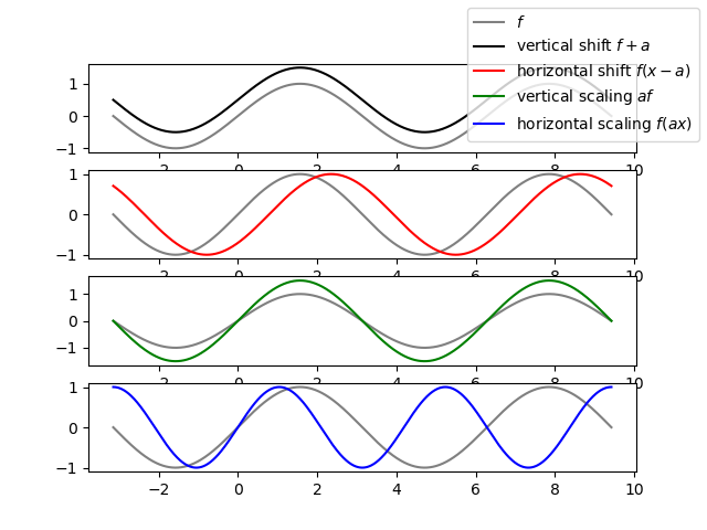
1.2.4. Scaling and Shifting Functions

In this section we set

\[f(x) = \sin(x)\]

as the example to illustrate shifting and scaling functions. First the definitions of shifting and scaling.

Definition 1.2.10 (Vertical Shift)

The function \(g(x)=f(x)+a\) is the function \(f\) shifted vertically over distance \(a\).

Definition 1.2.11 (Vertical Scaling)

The function \(g(x)=a f(x)\) is a vertically scaled version of \(f\).

Definition 1.2.12 (Horizontal Shift)

The function \(g(x) = f(x-a)\) is a horizontally shifted version of the function \(f\).

Definition 1.2.13 (Horizontal Scaling)

The function \(g(x) = f(ax)\) is a horizontally scaled version of \(f\).

These function transformations (a scaling or shift transformation takes one function as input and returns another function) are illustrated in the figure below.

Show code for figure

x = np.linspace(-np.pi, 3*np.pi, 1000)
f = np.sin(x)

fvshift = f + 0.5
fhshift = np.sin(x-np.pi/4)
fvscale = 1.5 * f
fhscale = np.sin(1.5*x)

fig, axs = plt.subplots(4)

axs[0].plot(x, f, color='gray', label=f"$f$")
axs[0].plot(x, fvshift, color='black', label=f"vertical shift $f+a$")

axs[1].plot(x, f, color='gray')
axs[1].plot(x, fhshift, color='red', label=f"horizontal shift $f(x-a)$")

axs[2].plot(x, f, color='gray')
axs[2].plot(x, fvscale, color='green', label=f"vertical scaling $a f$")

axs[3].plot(x, f, color='gray')
axs[3].plot(x, fhscale, color='blue', label=f"horizontal scaling $f(ax)$")

fig.legend()
plt.savefig("source/images/fshiftscale.png")

1.2.5. Extrema of Univariate Functions

An extremum of a function is either a (local) maximum or a (local) minimum. In case \(f\) is differentiable at \(x\) an extremum is characterized by \(f'(x)=0\). This is a necessary condition but not a sufficient condition, an inflection point is also characterized with \(f'(x)\) but is neither a maximum nor a minimum. All points for which \(f'(x)=0\) are known as stationary points, stationary because for \(h\to0\), we have \(f(x+h)=f(x)\) (why?).

To distinguish between maximum, minimum and reflection points we need the second order derivative. We have:

Theorem 1.2.14 (Stationary Point Classification)

A stationary point is defined as a point \(x\) where \(f'(x)=0\).

A stationary point \(x\) is a local maximum in case \(f''(x)<0\).

A stationary point \(x\) is a local minimum in case \(f''(x)>0\).

A stationary point \(x\) is a reflection point in case \(f''(x)=0\).

1.2.6. Exercises

1. Calculate the derivatives, with respect to \(x\), of the following functions (a, b, c, .. are constant values). Indicate the differentiation rules that you have used.

   1. \(\sin(\cos(x))\)

   2. \(\ln(x^2)\)

   3. \(c e^{- a x^2}\)

   4. \(\ln(\cos(x^3))\)

2. Give a proof for the quotient rule using the product rule.

3. Suppose you have a function \(g(x) = f( h(x) )\), where you know \(h(x_0) = 2/3\) and \(h_x(x_0) = 3/4\) for some constant \(x_0\). What is the value of \(g_x(x_0)\) if \(f(x) = x^2\)?

4. Calculate the following integrals. Again \(a, b\) and \(c\) are constants:

   1. \[\int_0^1 a x^2 dx\]
   2. \[\int_{0}^{\pi} \sin(x) dx\]
   3. \[\int_{0}^{\pi} \cos(x) dx\]

      If you first plot the cosine function than the value of this integral should obvious without calculation. But nevertheless for practice you should do it with a calculation as well.

   4. What about

      \[\int_{-\tfrac{1}{2}\pi}^{\tfrac{3}{2}\pi} \sin(x) dx\]
   5. \[\int_{-\pi}^0 b \sin(x) dx\]
   6. \[\int_0^\infty c e^{-x} dx\]
   7. \[\int_0^\infty c \lambda e^{-\lambda x} dx\]

      with constant \(\lambda>0\)

5. Determine the value of \(a\) such that

   \[\int_0^1 a x^2 = 1\]

6. Calculate the integral

   \[\int_{0}^{x} e^{-y^2} dy\]

   You may try to find a primitive but you cannot. This integral is a non elementary integral, i.e. it cannot be expressed using only the elementary standard functions. Look for the \(\text{erf}\) or error function on wikipedia.

   Write the value of this integral using this \(\text{erf}\) function.

   The lesson to be learned that even quite nice functions not always have a primitive that can be written as a composition of elementary (standard) functions.

7. Calculate the derivative of \(g(x)\) in terms of the derivative of \(f(x)\) for

   1. \(g(x) = f(x) + a\)

   2. \(g(x) = f(x - a)\)

   3. \(g(x) = a f(x)\)

   4. \(g(x) = f(ax)\)

8. Given that \(F\) is a primitive of \(f\), then:

   1. What is the integral \(\int_b^c f(x)\) in terms of \(F\)?

   2. What is the integral \(\int_b^c g(x)\) in terms of \(F\) for \(g(x)=f(x)+a\).

   3. What is the integral \(\int_b^c g(x)\) in terms of \(F\) for \(g(x)=f(x-a)\).

   4. What is the integral \(\int_b^c g(x)\) in terms of \(F\) for \(g(x)=af(x)\).

   5. What is the integral \(\int_b^c g(x)\) in terms of \(F\) for \(g(x)=f(ax)\).

Footnotes

[1]

Well, not quite… Python neither uses call by reference (then the function is aware of the identity of the argument) nor call by value (then it is totally unaware of the identity). Read about call by object reference in case you want to know more.

[2]

Well… there is mathematical theory to handle these situations as well. Read about subdifferentials in case you are really interested. Actually the source code of PyTorch speaks about subdifferentials when differentiating the max function, illustrating the fact that machine learning does require some advanced math.

[3]

It looks like a proof, but really it is not. When saying that \(\sin(h)\rightarrow h\) when \(h\rightarrow0\) we are implicitly using the derivative of the sine function (as \(\sin(h)\approx h\) is the first order Taylor series approximation of the sine function. For a real proof see the Kahn Academy video

[4]

The animation of the limit in the Riemann definition of the integral is an animation based on the sum:

\[\sum_{i=0}^{n-1} f(x_i + \half dx) dx\]

but in the limit for nicely behaving functions this is not significant and will lead to the same answers.