2.6. Probability Distributions

There are a lot of probability mass functions and probability density functions for which an analytical expression is known. These functions are parameterized in the sense that only a few parameters define the value for every value \(x\).

In this section we discuss some of the most often used functions. In a later section we describe one method to estimate the parameters given a sample from a distribution.

2.6.1. Discrete Distributions

A discrete distribution is completely characterized with its probability mass function \(p_X\). Remember that for a probability mass function we should have that the sum over all possible outcomes \(x\) equals 1 and that all probabilities are greater than or equal to zero. Given that function we will calculate (or only give the result) both the expectation and the variance.

2.6.1.1. Bernoulli Distribution

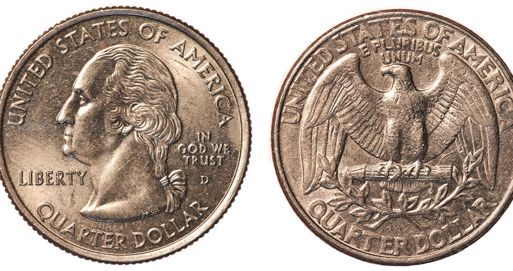
Fig. 2.6.1 Heads or Tails. Grammarist explains. “Heads refers to the side of the coin with a person’s head on it. Tails refers to the opposite side, not because there is a tail on it, but because it is the opposite of heads.”

The simplest of all probabilistic experiments perhaps is tossing a coin. The outcome is either heads or tails, or 0 or 1. Such an experiment is called a Bernoully experiment and the corresponding distribution is called the Bernoulli distribution.

The Bernoulli distribution has parameter \(p\). In case the random variable \(X\) is Bernoulli distributed we write \(X\sim\Bernoulli(p)\).

The probability mass function is:

\[\begin{split}p_X(x) = \begin{cases} 1-p &: x=0\\ p &: x=1\\ 0 &: \text{elsewhere} \end{cases}\end{split}\]

The expectation equals:

\[\begin{split}\E(X) &= \sum_{x=-\infty}^{\infty} x\,p_X(x)\\ &= 0\times (1-p) + 1\times p\\ &= p\end{split}\]

and its variance:

\[\Var(X) = p(1-p)\]

2.6.1.2. Binomial Distribution

Fig. 2.6.2 Galton Board. A simulation of a Galton board. The distribution of the ball over the bins follows binomial distribution. Open the animated gif image in a separate window to clearly see the pins that force a falling ball to go either left or right (the Bernouilli experiment). Google for Galton board video and you can see a physical Galton board in action.

Consider a Bernoulli distributed random variable \(Y\sim\Bernoulli(p)\), and let us repeat the experiment \(n\) times. What then is the probabilty of \(k\) successes. A success is defined as the outcome \(Y=1\) for the Bernoulli experiment.

So we define a new random variable \(X\) that is the sum of \(n\) outcomes of repeated independent and identicallu distributed (iid) Bernoulli experiments.

The outcomes of \(X\) run from \(0\) to \(n\) and the probability of finding \(k\) successes is given as:

\[p_X(k) = P(X=k) = {n \choose k}\,p^k\,(1-p)^{n-k}\]

This is called the Binomial Distribution. For a random variable \(X\) that has a binomial distribution we write \(X\sim\Bin(n,p)\).

The expectation is:

\[\E(X) = n\,p\]

and the variance:

\[\Var(X) = n\,p\,(1-p)\]

Show code for figure

import numpy as np
import matplotlib.pyplot as plt

from scipy.stats import binom

n = 20
for p, c in zip([0.05, 0.4, 0.8], ['r', 'g', 'b']):
    plt.stem(np.arange(0, n+1), binom.pmf(np.arange(0, n+1), n, p),
             linefmt=c, markerfmt=c+'o',
             label=f'p={p}')

    plt.legend()
plt.xticks(np.arange(0, n+1))
plt.savefig('source/figures/binomialdistribution.png')

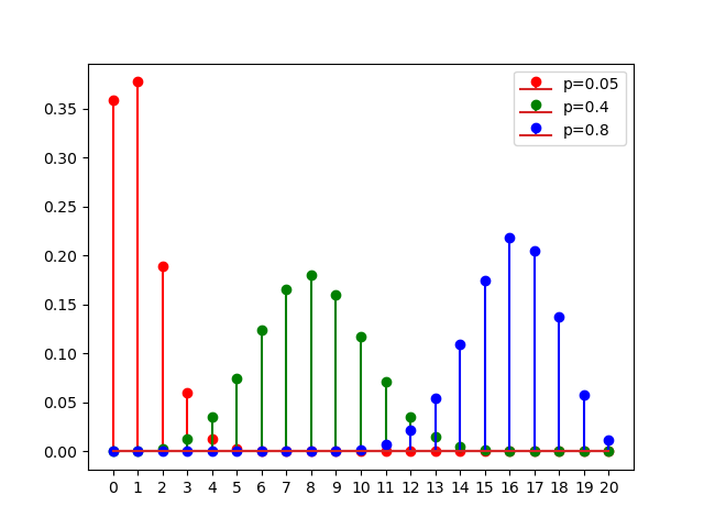
Fig. 2.6.3 Binomial Distribution. Shown are the binomial probability mass functions for \(n=20\) and \(p\in\{0.05, 0.4, 0.8\}\).

2.6.1.3. Uniform Distribution

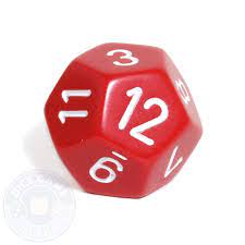
Fig. 2.6.4 Twelve sided die. Throwing this die result in a number in the range from 1 to 12 to show on top with equal probability (in case of a fair die).

The discrete uniform distribution is used in case all possibe outcomes of a random experiment are equally probable. Let \(X\sim\Uniform(a,b)\), with \(a<b\) and \(a,b\in\setZ\), then

\[\begin{split}p_X(x) = \begin{cases} \frac{1}{b-a+1} &: a\leq x \leq b\\ 0 &: \text{elsewhere} \end{cases}\end{split}\]

Its expectation is:

\[\E(X) = \frac{a+b}{2}\]

and its variance

\[\Var(X) = \frac{(b-a+1)^2-1}{12}\]

2.6.2. Continuous Distributions

2.6.2.1. Uniform Distribution

The continuous uniform distribution characterizes a random experiment in which each real valued outcome in the interval \([a,b]\subset\setR\) is equally probable. The probability density function of \(X\sim\Uniform(a,b)\) is given by

\[\begin{split}f_X(x) = \begin{cases} \frac{1}{b-a} &: a \leq x \leq b\\ 0 &: \text{elsewhere} \end{cases}\end{split}\]

The expectation of the continuous uniform distribution is

\[\E(X) = \frac{a+b}{2}\]

and its variance

\[\Var(X) = \frac{(b-a)^2}{12}\]

2.6.2.2. Normal Distribution

The normal distribution is undoubtly the most often used distribution in probability and machine learning. For good reasons: a lot of natural phenomena of random character turn out to be normally distributed (at least in good approximation). Furthermore the normal distribution is a nice one to work with from a mathematical point of view.

Let \(X\sim\Normal(\mu,\sigma^2)\) then the probability density function is:

\[f_X(x) = \frac{1}{\sigma\sqrt{2 \pi}} e^{-\frac{(x-\mu)^2}{2\sigma^2}}\]

where the parameters \(\mu\) and \(\sigma^2\) are called the mean and variance for obvious reasons:

\[\begin{split}&\E(X) = \mu\\ &\Var(X) = \sigma^2\end{split}\]

There is no analytical expression for the cumulative distribution function \(F_X\) for \(X\sim N(0,1)\) (nor for any normal distribution). We Instead we write:

\[F_X(x) = \frac{1}{2}\left(1+\text{erf}\frac{x}{\sqrt{2}}\right)\]

where \(\text{erf}\) is the error function

\[\text{erf}(x) = \frac{2}{\sqrt{\pi}} \int_0^x e^{-t^2} dt\]

The error function is available in Numpy as scipy.special.erf. Given \(F_X(x)\) we can easily calculate the probability for any outcome in the interval from \(a\) to $b%:

\[\P(a\leq x \leq b) = F_X(b) - F_X(a)\]

Famously we have:

\[\begin{split}\P(\mu - \sigma\leq &x \leq \mu+\sigma) = 0.683\\ \P(\mu - 2\sigma\leq &x \leq \mu+2\sigma) = 0.954\\ \P(\mu - 3\sigma\leq &x \leq \mu+3\sigma) = 0.997\end{split}\]

which are illustrated in the figure below:

Show code for figure

import numpy as np
import matplotlib.pyplot as plt
from scipy.special import erf

def Phi(x):
    return 0.5 * (1 + erf(x / np.sqrt(2)))

def phi(x):
    return 1/np.sqrt(2*np.pi) * np.exp(-x**2/2)

fig, axs = plt.subplots(3)
x = np.linspace(-4, 4, 1000)

for i, s in enumerate([1,2,3]):
   axs[i].plot(x, phi(x))
   xi = x[np.logical_and(x>-s, x<s)]
   axs[i].fill_between(xi, 0, phi(xi))
   axs[i].text(2, 0.3, "P = {P:5.3f}".format(P=Phi(s)-Phi(-s)))
   plt.axhline(0)

plt.savefig('source/figures/normalintervals.png')

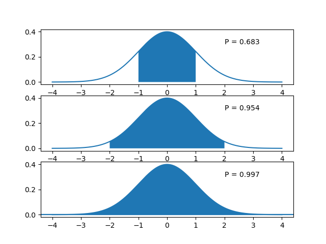
Fig. 2.6.5 Normal Distribution. Shown are the intervals from \(\mu-k\sigma\) to \(\mu + k\sigma\) and their probability \(\P(\mu-k\sigma\leq x \leq \mu+k\sigma)\) for \(k=1,2,3\).