2.1. Probability Space and Probability Axioms
2.1.1. Random Experiments and Probability Spaces
To describe a random experiment in mathematical terms we need what is called a probability space. Such a space consists of three things:
The set of all possible outcomes of the random experiment. We will denote this set as \(U\) for universe.
A collection of subsets of \(U\). A subset \(A\) if \(U\) (i.e. \(A\subset U\)) corresponds with an event. For example when throwing a die a possible event is to throw a 6. Another possibiliy is the event corresponding with throwing an odd number of points.
A probability measure \(\P\) that maps each subset \(A\subset U\) (event) onto a positive scalar \(\P(A)\)
2.1.2. Probability Axioms
Let \(A\) and \(B\) both be subsets of the probability space (the universe) \(U\), i.e. \(A\) and \(B\) are events. Surprisingly maybe, the whole theory of probability is based upon just three axioms:
The first axiom simply states that probabilities are non negative (real) numbers.
The second axioma states that the probability for the universe \(U\) equals 1. This is intuitively clear as the universe contains everything that could ever happen.
The third axiom is the only axiom that relates probabilities of several events: if event \(A\) and event \(B\) are mutually exclusive (i.e. you can’t have \(A\) and \(B\) being the simulatanuous outcome of one random experiment, e.g. throwing with a die and having events “6” and “odd”) then the probability of either event \(A\) or event \(B\) occuring, i.e. \(A\cup B\), equals the sum of \(\P(A)\) and \(\P(B)\).
2.1.3. Venn Diagrams
To gain insight and some intuition of probability space it is useful to depict that space as a two dimensional subset of the plane (the Venn diagrams of sets).
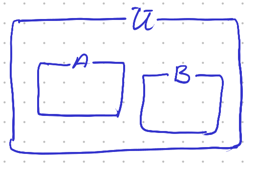
Fig. 2.1.1 Disjunct sets. The sets \(A\) and \(B\) have nothing in common, i.e. \(A\cap B=\emptyset\).
Consider the Venn diagram corresponding with the third axiom. We have the universe \(U\) and the two events \(A\) and \(B\), both subset of \(U\). The assumption that \(A\cap B =\emptyset\) is visualised as the empty intersection of the two sets.
You may take the visual interpretation somewhat further and assume the relative area of set \(A\) with respect to the area of set \(U\) corresponds with the probability \(\P(A)\):
Please note that this is NOT the definition of \(\P(A)\) ! It is stating the rule to interpret the Venn diagrams.
2.1.4. Simple Probability Theorems
The definitions and axioms in a mathematical theory are the starting point, but the interesting parts are the theorems, the things that can be proven to be true given the definitions and the axioms. Probability theory is no exception.
Let us start with a simple definition: the complement. Let \(A\) be an event, i.e. subset of \(U\). Then we define the complement \(\neg A\) as:
where \(\setminus\) denotes the ‘set minus’, i.e. everything in the universe that is not in \(A\). This is just a definition. A theorem however is the statement:
The proof obviously needs the third axiom as we have to relate the probabilities of two events: \(A\) and \(\neg A\). Observe that:
By definition we have that \(A\) and \(\neg A\) are disjunct, i.e. \(A\cap \neg A=\emptyset\), and thus we can utilize the third axiom:
Using the second axiom and rewriting the equation we get:
and that completes the proof.
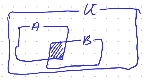
Fig. 2.1.2 Intersection of sets. The intersection \(A\cap B\) is sketched as the hatched area.
Now consider the situation where events \(A\) and \(B\) are not disjunct. Then we cannot apply the third axiom directly. Look at a Venn diagram of two subsets \(A\) and \(B\) or \(U\) with non empty intersection. From such a figure it is intuively clear that
The proof is simple as well. We leave that to the reader in an exercise.