Chapter 3 Uncertainty
3.1 Recap
In Chapter 1 we learned how to formulate statistical models to describe our data and in chapter 2 we learned how to fit these models to data. The estimated parameter values then can give us useful information related to a scientific question, for example, what is the relationship between GDP and carbon emissions among countries? Or what is the effectiveness of a vaccine relative to a control?
We can attempt to answer these questions by fitting statistical models to data. For example, we one wanted to study the effectiveness of a drug for reducing the blood pressure of patients with elevated blood pressure, we might design a study where we give patients either the drug or a placebo and then measure blood pressure after some time on the medication. For now, lets assume that there is no patient information we want to include in my statistical model, and the only independent variable is the treatment (drug or placebo).
\[ y = b_0 + b_1 x \] where \(y\) is blood pressure and \(x = 0\) if patients were given the placebo and \(x = 1\) if patients were given a drug.
Problem 3.1 If you were interested in testing the hypothesis that the drug is more effective than a placebo for patients with high blood pressure, which parameter would be of interest?
\(b_1\) is the estimated difference in blood pressure between treatments (would be negative if the drug reduces blood pressure).
Let’s say you fit this model to your data and estimate \(b_1\) to be -5.1 mmHg. This means that patients that were prescribed the drug had on average a blood pressure that was 5.1 mmHg lower than patients prescribed the placebo. If this study had collected data for every person with high blood pressure in the world (the population of interest), we could probably stop here. However for almost any real study, we don’t have data for the entire population, instead, we try make inferences about the population of interest from a smaller sample of that population. Instead of including every person with high blood pressure, we might try to get a representative sample of 100 individuals with high blood pressure. Working with samples instead of populations makes doing science feasible, but it also introduces a new problem: uncertainty. Some patients might be helped a lot by the drug, some not as at all. As a result, if we repeated our study, we would get a slightly different answer every time due to the randomness of who happens to be in our study. It also means that the estimated effect of the drug we get from our study will also be different from the true average effectiveness of the drug if we sampled the entire population of interest. The difference between our estimate from our sample, and the true population parameter is called the sampling error. This means that whenever we use samples to infer things about a population, we do so with some error and uncertainty. An important problem we use statistics for is then to estimate how uncertain our estimates and conclusions are given the randomness imposed by finite sample sizes. But how do we do this?
3.2 The sampling distribution and the Central Limit Theorem.
A sampling distribution is a hypothetical distribution of parameter estimates we would get if we repeated our study an infinite number of times. The best way to get intuition for sampling distributions (and many other concepts in statistics) is through simulation. We will illustrate the sampling distribution with an example.
In this example, we want to estimate the average height of students at UvA from a random sample of a small number of students. In this example, we aren’t trying to explain student height as a function of any other variables, so our model is just:
\[ \hat y = b_0 \]
Let’s assume that the true average height of UvA students is 170 cm with a standard deviation of 10 cm. The question is then, is how accurate are our estimates of this true population parameter for a given sample size?
The smallest sample size possible is 1. In this case we just randomly select a student, record their height, and then our estimate for the mean height of UvA students is equal to the height of the randomly selected individual. In this case our estimate of the mean UvA student height will be as variable as the individuals in the population.
We can write an R program to simulate a large number of studies where we randomly draw one student from the population, and record their height, take the mean (which with a sample size of 1 just equals the height of the selected student). We use a for loop to repeat this many times (10000):
sample_size = 1
N_studies = 10000 # a large number to approximate infinite number of studies
sample_mean = rep(NA,N_studies)

# repeat the study many times
for (i in 1:N_studies){
sample_mean[i] <-mean(rnorm(sample_size,170,10))
}
In the code above, sample_mean is a vector that contains the results of each of the 10000 studies we conducted, each measuring the height of one student. We simulated this in our code by using the rnorm() function in R, to draw 1 observation from the population distribution with mean 170 and standard deviation of 10.
If we plot out the distribution of the estimates along with the probability density function for the population we see that they are essentially identical:
hist(sample_mean,freq=F,breaks=50,xlim=c(140,200))
x<-seq(100,200,length.out = 100)
pdf<-dnorm(x,170,10)
lines(x,pdf)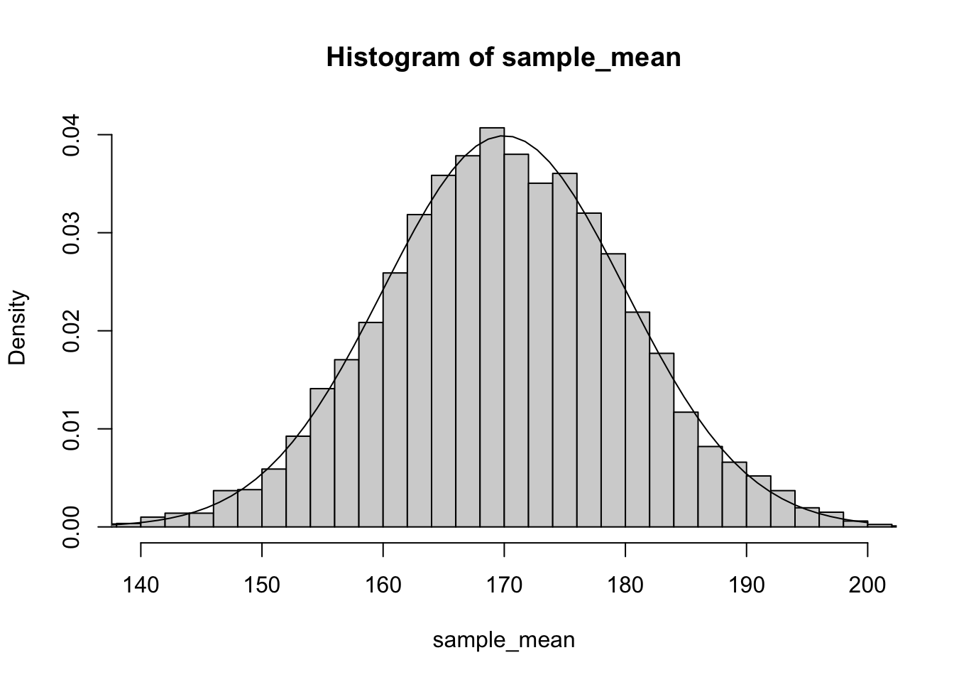
As you can see the estimates of our studies are highly variable when we only have a sample size of 1. If we happen to pick 1 unusually short or tall person, our estimate can be off by as much as 20 cm. To improve the precision of our estimate we could sample multiple individuals. For example, if we increased the sample size to 5, we see that our estimates of average height become much less variable:
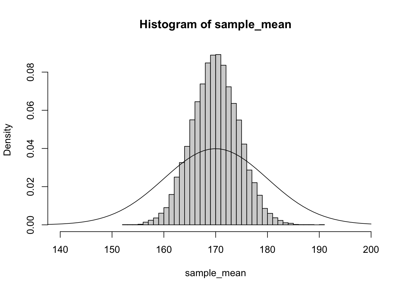
and if we further increased the sample size to 20, the distribution of estimates of average height is even less variable:
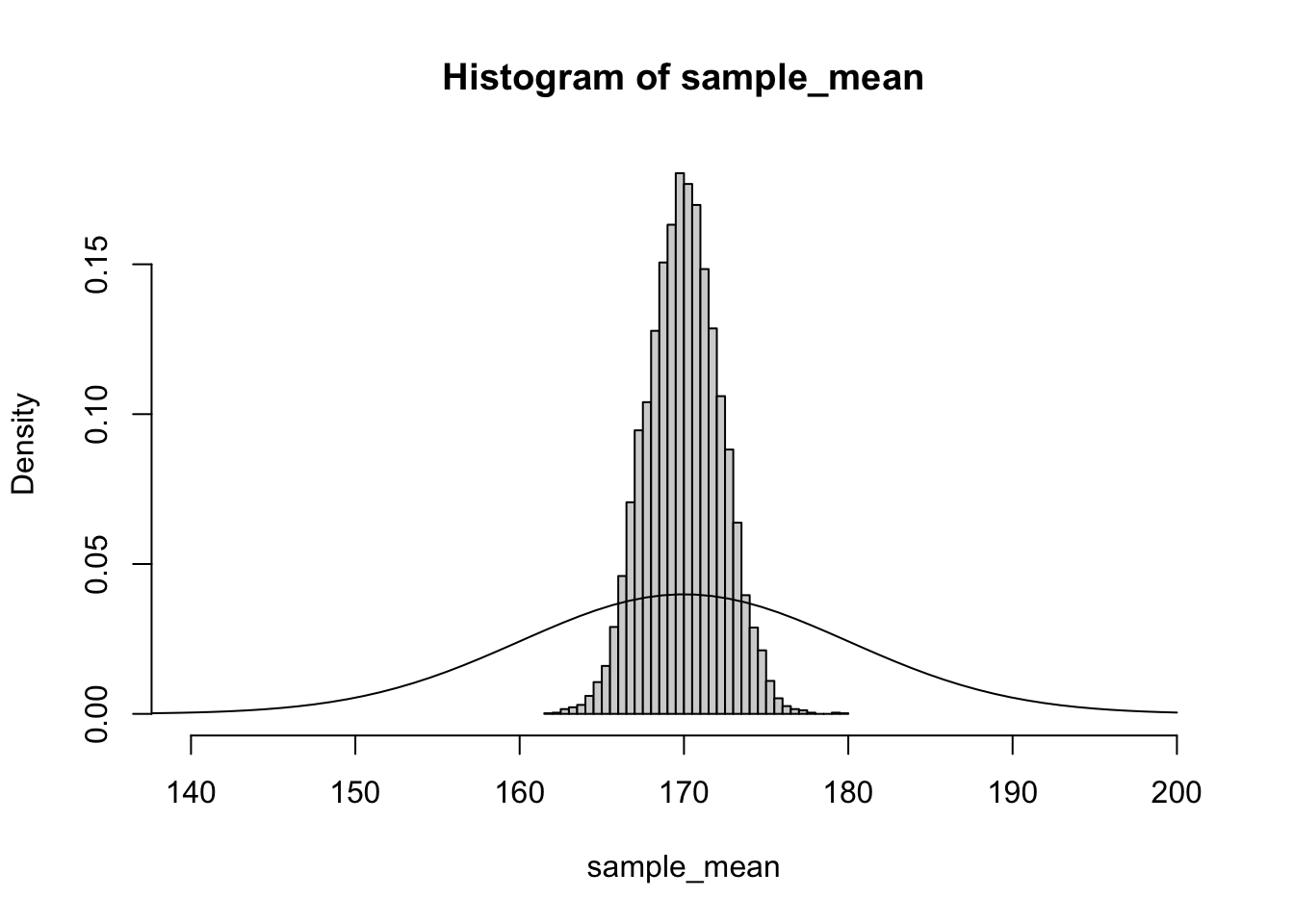
The intuition for why this happens is that as you take multiple samples, it becomes more and more likely for the extreme values to cancel each other out. While it might not be that unlikely to randomly select a student that is over 190 cm (around 1 in 10 chance), it would be very unlikely to randomly select 5 students who were all over 190cm (\(0.1^5\) = about 1 in 100000 chance). Thus as we take larger samples, our estimate of the average height of students at UvA more closely approximates the true population parameter.
An important point about sampling distributions is that for continuous variables they are approximately normally distributed. In the histogram plots above you can see clearly that they look almost exactly like a normal distribution.
Because sampling distributions are approximately normal, we can quantify the shape of the distribution by its standard deviation. The standard deviation of the sampling distribution tells us how variable the estimates of a model parameter are across replicate studies. In the UvA height example, we have the model parameter \(b_0\), which is just the mean of the sample. The standard deviation of the sampling distribution for \(b_0\) is referred to as the standard error of the parameter estimate. In this context, because the parameter is a sample mean, it is also referred to as the standard error of the mean. But in general every estimated parameter in our model has sampling error, and the standard error of the parameter tells us how uncertain our estimate of that parameter is. When the standard error is very large, it means that the estimate of the parameter values is highly uncertain and the true population parameter may be quite different from the estimated parameter from a sample.
Interestingly, if you have a large enough sample size (~30 or more), the sampling distribution will approximate a normal distribution even if the raw data are not normally distributed. This result is known as the Central Value Theorem. In class we will show an example of how normal distributions emerge from averages of highly skewed data. The Central Value Theorem is really an astonishing and surprising result with some important implications. First it means that even when the raw data don’t have normally distributed errors, the sampling distribution of parameters (for example a mean or regression slope) will be approximately normal. Thus our estimates of standard errors and confidence intervals are still approximately valid even when the raw data is not normal (assuming large enough sample sizes). Secondly, the Central Value Theorem helps explain why so many variables turn out to be normally distributed. Whenever a variable like someones’ height, is determined by the aggregate effect of many random variables (e.g. many genes and environmental factors) the variable will be approximately normally distributed.
3.3 How does uncertainty in parameter estimates change with sample size?
How large does our sample size need to be to accurately estimate the population parameters of interest?
We can begin to answer this question by repeating our analysis for different sample sizes. In the code below I use an additional for loop to generate sampling distributions for sample sizes ranging from 1 to 200. For each sample size I then calculate the standard deviation of the sampling distribution (the standard error of a parameter estimate) and then plot it as a function of sample size:
sample_size = round(seq(1,200,length.out=40))
N_studies = 10000 # a large number to approximate infinite number of studies
sample_mean = rep(NA,N_studies)
standardError = rep(NA,length(sample_size))
# repeat study many times
for (j in 1:length(sample_size)){
  for (i in 1:N_studies){
    sample_mean[i] <-mean(rnorm(sample_size[j],170,7))
  }
standardError[j]=sd(sample_mean)
}
plot(sample_size,standardError)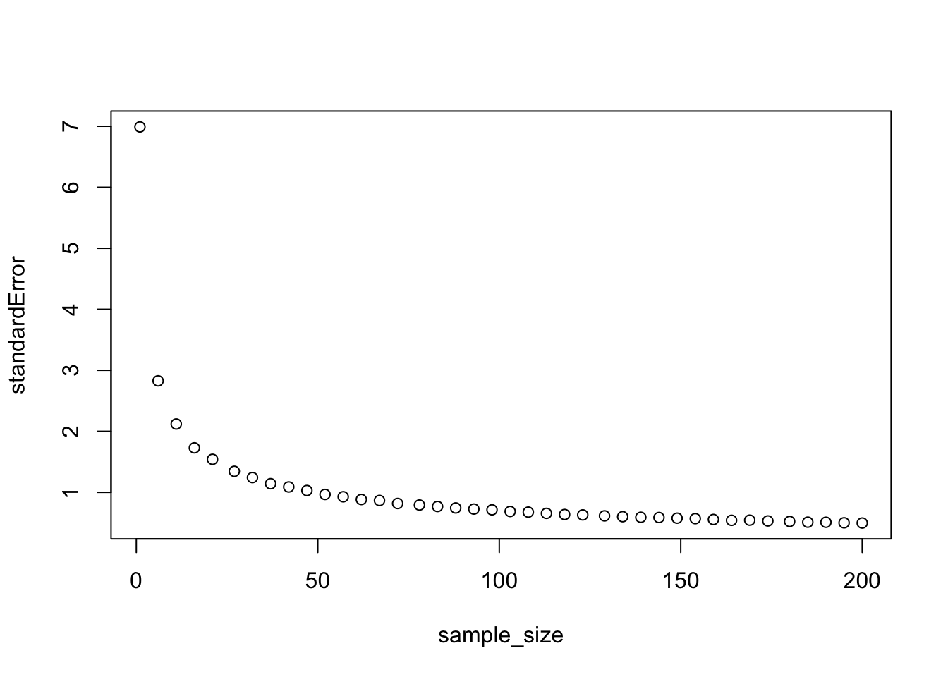
As you can see the standard error goes down with sample size, but with diminishing returns. Standard error decreases more rapidly with sample size when sample size is low.
3.4 Calculating standard errors from a sample
In the example above, we could calculate standard errors of parameter estimates by simulating a study many, many times. But in the real world, we generally just have one study. Fortunately, we can estimate the standard error of parameters directly from a sample. In the case of a model with no independent variables (just a mean) there is a simple formula to calculate the standard error of the mean:
\[ \hat{SEM} = \hat\sigma/\sqrt{n} \] where \(\hat\sigma\) is the residual standard error (the estimated standard deviation of the residuals or error) and \(n\) is the sample size.
For more complex models with multiple parameters, there isn’t a simple formula to calculate standard errors, it requires linear algebra, but the essence of this formula holds also for more complex models. The standard error of parameter estimates will increase as the data becomes noisier (larger \(\sigma\)) and the standard error of parameters will decrease with increasing sample size, but again with diminishing returns.
When you fit a model to data in R or any other statistical software, it will return the parameter estimate for each parameter in the model, but also the standard error for each parameter value. The parameter estimate tells you the most likely value of the parameter given the data, and the standard error tells you how wide the range of likely values are for the parameter. If a parameter has a large standard error that means that there is a lot of uncertainty about the true population parameter, while if the standard error is small, then it suggests that the true population parameter is likely very close to the estimated value.
Going back to the CO2 emissions data set:
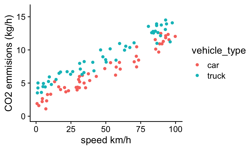
We can fit a model with two independent variables (speed and vehicle_type) to the data using the lm() function:
Call:
lm(formula = CO2 ~ speed + vehicle_type, data = df)

Residuals:
     Min       1Q   Median       3Q      Max
-2.52676 -0.45656  0.02895  0.58776  1.96606

Coefficients:
                  Estimate Std. Error t value Pr(>|t|)
(Intercept)       1.897667   0.167456   11.33   <2e-16 ***
speed             0.100947   0.002557   39.49   <2e-16 ***
vehicle_typetruck 2.145354   0.162546   13.20   <2e-16 ***
---
Signif. codes:  0 '***' 0.001 '**' 0.01 '*' 0.05 '.' 0.1 ' ' 1

Residual standard error: 0.8124 on 97 degrees of freedom
Multiple R-squared:  0.9478,    Adjusted R-squared:  0.9468
F-statistic: 881.3 on 2 and 97 DF,  p-value: < 2.2e-16
In the “coefficients” section of summary table of the model, there are 3 rows. Each row corresponds to a parameter in the model, with the name of the parameter to the left of the table. In the table the first column shows the parameter estimate, and the 2nd shows the standard error. For now we will ignore the other columns. You should be able to look at the first two rows and get an idea of the likely range of the true population parameters.
Problem 3.2 Plot out the estimated probability density function for the parameter associated with vehicle_type (truck = 1).
We can answer this question using the dnorm() function and plugging in the parameter estimate for vehicle_typetruck and its standard error:
vehicle_typetruck<-seq(0,4,length.out=200)
density<-dnorm(vehicle_typetruck,1.907,0.164)
plot(vehicle_typetruck,density,'l')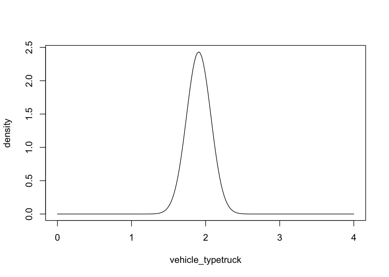
Problem 3.2 By looking at this figure above, we can see that the most likely value is a little less than 2. If you had to estimate by eye, what is the minimum value for the population parameter that seems likely? What about the maximum value?
With this problem I am asking you about your confidence that the true population parameter of the difference in mean CO2 emissions of trucks vs. cars falls within some bound. For example, you might want to say something like, the estimated difference in CO2 emissions in trucks vs. cars is 1.9, and I am 95% confident that the true difference between trucks and cars (if we collected data for every car and truck in the world) would be between 1.5 and 2.3. What I just described is a confidence interval. Here, I just guessed these values by eyeballing the figure, but below we will show how they can be calculated precisely. However before doing so, we first need to review the relationship between probability density functions and probabilities.
3.4.1 Review of probability density functions and probabilities
The plot above is another example of a normal probability density function. As a reminder, the integral of a pdf over the entire range of possible values, or the total area under the curve, equals 1. Moreover if we specify any range on this continuous scale, by a lower and upper value, the area under the curve between these two points is the probability the value falls within this range.
For example, if we have a random variable, \(y\), with mean 0 and sd = 1:
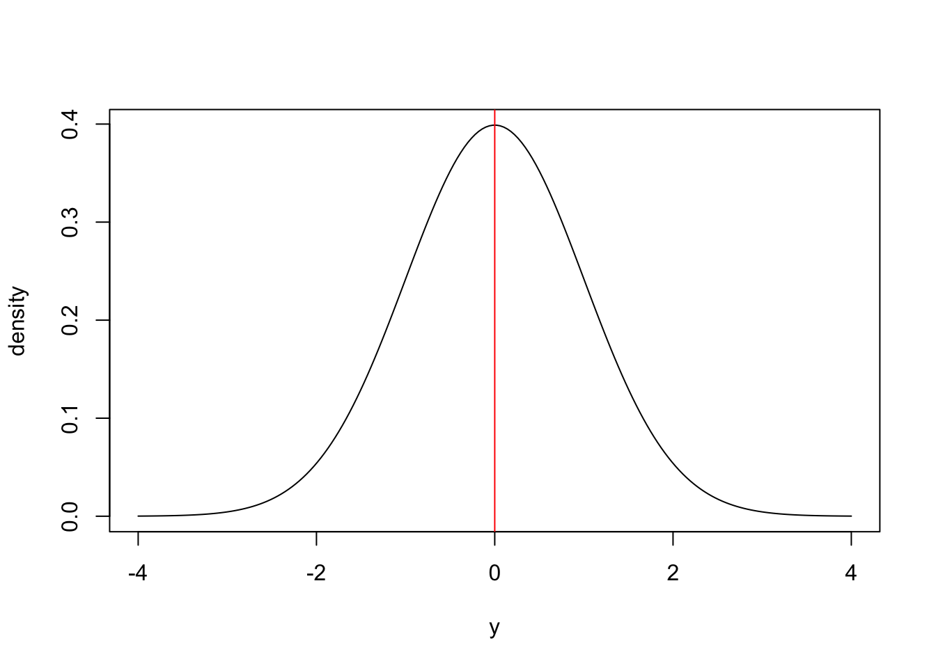
the distribution is symmetric around the mean, with half the area under the curve occurring for values \(y < 0\) and half the area under the curve for values of \(y\) above zero. Thus the probability of drawing a random number greater than zero would be 50%. We might also want to know what is the probability of an observation falling within some distance of the mean? For example, what fraction of observations drawn from a normal distribution do we expect to fall within 1 standard deviation of the mean. This is essentially asking the question what proportion of the total area under the curve occurs between -1 and 1 times the standard deviation (between -1 and 1 sd) from the mean. It turns out that approximately 68% percent of the area under the curve falls within 1 standard deviation of the mean:
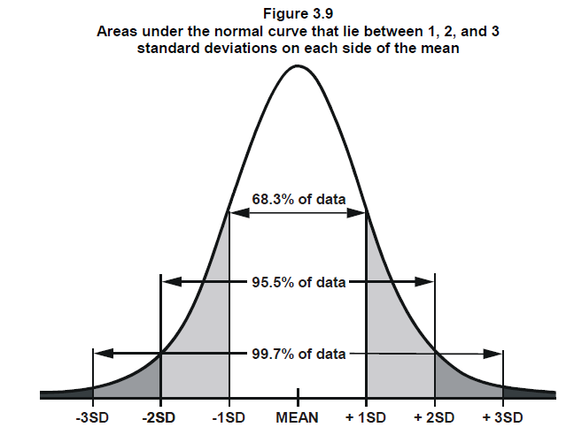
You can also see that 95% percent of the area under the curve is within 2 standard deviations of the mean, and nearly all, 99.7% of the area under the curve is within 3 standard deviations of the mean.
We can calculate these numbers precisely using the pnorm() function in R. The syntax of pnorm is:
pnorm(x = 0, mean = 0, sd = 1)pnorm() returns the integral (area under the curve) from -infinity up to the value of \(x\) in the first argument for a given mean and standard deviation sd. So the probability of observing a value of \(x\) less than zero when mean = 0 and sd = 1 can be computed with:
[1] 0.5And the probability of observing a value less than -1 as:
[1] 0.1586553Because the normal distribution is symmetric the probability of observing a value less than -1 times the standard deviation is the same as the probability of observing a value greater than 1 times the standard deviation. So the probability of observing a value between -1 and 1 is:
[1] 0.6826895which agrees with the approximate value stated earlier.
Problem 3.3 If \(y\) is a normally distributed random variable with mean 2.1 and standard deviation 1.3, what fraction of \(y\) values would you expect to fall between 0 and 1?
Plugging in the values we would expect:
[1] 0.05311371about 5% of the data to be less than 0, and:
[1] 0.1987335around 20% of the data to be less than 1, so \(20 - 5 \approx 15\)% of the data would be between 0 and 1.
Finally, if we plug in a vector of \(x\) values and plot the output of pnorm():
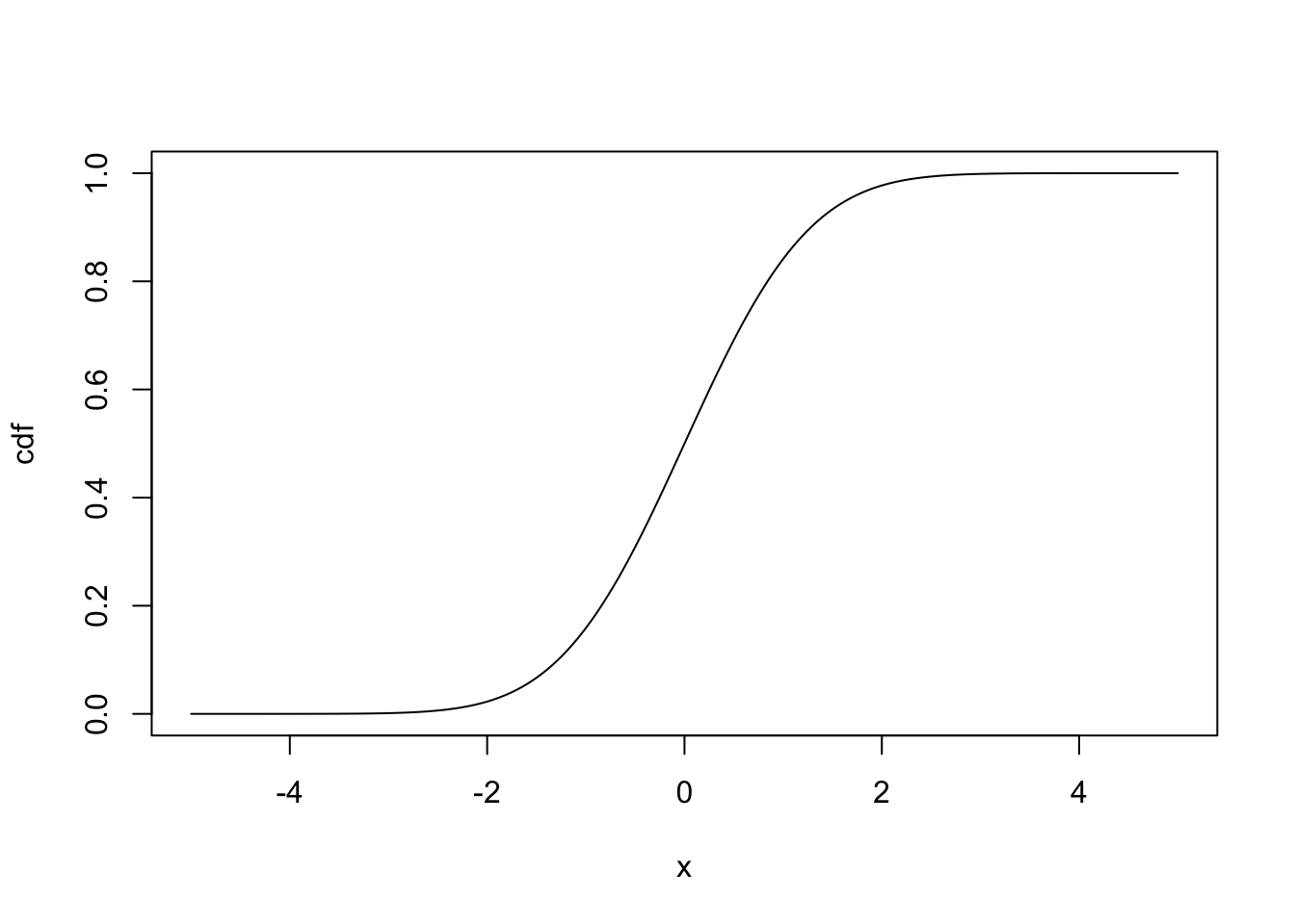
we see a cumulative distribution function, where the \(y\) value for a given \(x\) value corresponds to the probability of observing a value less than \(x\). You can see that the slope of the line increases most rapidly around the mean, because the slope of this line is equal to the probability density function, which is highest around the mean.
3.5 Confidence intervals
If you understand probability density functions and cumulative distribution functions, then confidence intervals are fairly straightforward. When you fit a model, you get a parameter estimate and standard error for each parameter. These two values can be used to produce a probability density function of the likely values of the parameter, and from this pdf we can calculate what interval is required to encompass 95% of the area under the curve.
The main distinction between confidence intervals and other applications of pdfs, is that confidence intervals don’t tell you the probability that the true population parameter falls within the confidence interval. This is because the true population parameter is a fixed value. For example in the context of the vehicle CO2 emissions, the true population parameter for “vehicle_type” is the average difference in CO2 emissions between trucks and cars, if we measured emissions for every car and truck. It has one specific value, and it either is or is not within out confidence interval. In our study, we tried to estimate the population value with a random sample of cars and trucks. If we repeated our study many, many times, in the long run we should expect the true population parameter to fall within the 95% confidence intervals about 95% of the time. Thus for any one sample, we can be 95% ``confident’’ that the true population parameter falls within our confidence intervals.
3.6 The 2 SE method for estimating 95% CI
Because approximately, 95% of the area under a normal distribution falls within 2 standard deviations of the mean, one quick (but approximate) way to estimate 95% confidence intervals is:
upper_CI = estimate + 2 sd
lower_CI = estimate - 2 sd
I call this ``the 2 SE method’’ for estimating 95% confidence intervals. The values produced by this method are not precise, but are generally very close, and this method is an easy way to look at parameter estimates and standard errors and get a sense for the range of likely parameter values.
We can calculate confidence intervals for data manually using data from the coefficients table from the summary output of the model:
                   Estimate  Std. Error  t value     Pr(>|t|)
(Intercept)       1.8976667 0.167455988 11.33233 1.838625e-19
speed             0.1009468 0.002556536 39.48578 1.421217e-61
vehicle_typetruck 2.1453539 0.162546470 13.19840 2.214078e-23
where mod is the name we use for the output of the lm() model fit.
If we want to access specific elements in the table we just need to specify the row and column number. For example the standard error of the intercept parameter is in the first row and 2nd column so we can access it by:
[1] 0.167456Problem 3.4 Use the quick and dirty 2 SE method to calculate the 95% confidence intervals for the parameter associated with vehicle_type.
You can easily do this manually, but using R you can do this by:
estimate = summary(mod)$coefficients[3,1]
s_e = summary(mod)$coefficients[3,2]
upper_CI = estimate + 2 * s_e
lower_CI = estimate - 2 * s_e

upper_CI
[1] 2.470447[1] 1.820261If we wanted to be more precise, we can use the qnorm() function to find the range of values needed to encompass 95% of the area under then normal curve. The ‘q’ stands for ‘quantile function’ and is the inverse function of pnorm(). For example if we have a normal distribution with mean = 0, sd = 1, we can calculate the probability of observing data less than -2 by:
[1] 0.02275013Which means that 0.0227 of the area under the curve occurs at values less than -2.
Conversely, if we ask what is the value of $xS below which 0.02275 of the area under the curve falls, we can use qnorm():
[1] -2So if you want to calculate how wide of an interval is needed to encompass 95% of the area under the normal distribution you would use qnorm:
[1] -1.959964 1.959964I used c(0.025, 0.975), because for 95% CI, 2.5% of the area under the curve will be on the lower tail, and 2.5% will be in the upper tail. Thus we see that the quick and dirty 2 SE rule is only approximate, the exact value is closer to 1.96. We can then use this value to calculate confidence intervals:
estimate = summary(mod)$coefficients[3,1]
s_e = summary(mod)$coefficients[3,2]
upper_CI = estimate + 1.96 * s_e
lower_CI = estimate - 1.96 * s_e

upper_CI
[1] 2.463945[1] 1.8267633.7 The t-distribution
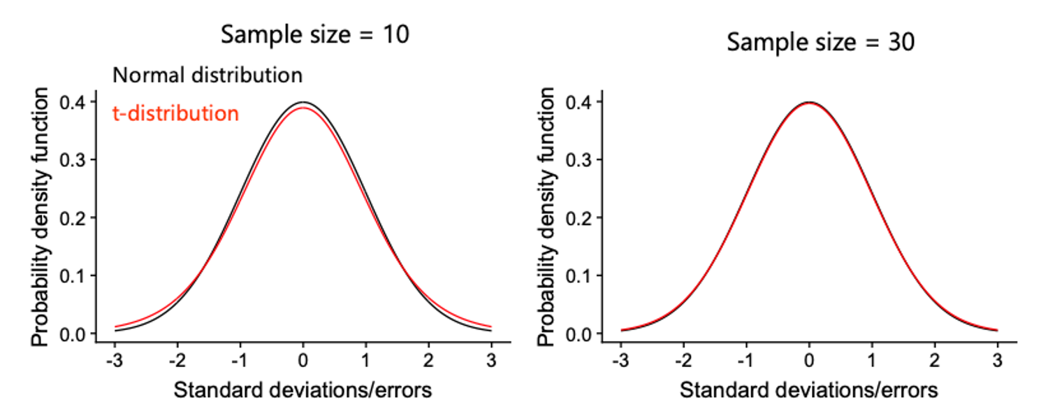
Now you should have the basic idea of confidence intervals and where they come from. However there is one more minor detail. The calculations we used assume that the \(\sigma\), the standard deviation of the errors is known, when in fact we just estimate it from our sample. The consequences of this is that to calculate the true confidence intervals, we have to use the t-distribution instead of the normal distribution. The t-distribution looks almost exactly like the normal distribution but it has wider tails. The shape of the distribution is also dependents on the amount of data we have, or more precisely the degrees of freedom. When we have lots of data (e.g. > 30 df) the t-distribution is almost indistinguishable from the normal distribution. It is only when we have very little data, that the distributions differ significantly. This is because when we have little data, there is more uncertainly about how variable the errors truly are.
 In the case of the vehicle CO2 emissions, we had 100 data points and 3 parameters, so 97 degrees of freedom. To calculate CI intervals using the t-distribution we need to calculate what interval on the t-distribution is needed to contain 95% of the area under the curve. For this we use the
 qt() function, which is like the qnorm() function but for the t-distribution instead of the normal distribution:
[1] -1.984723 1.984723Here the first argument is the same as in qnorm(), and the second argument is the degrees of freedom. We see the the values we get are very similar to qnorm(), because in this case we have a lot of data. If we only had 5 degrees of freedom, you see that the interval would be wider and thus so would the confidence intervals:
[1] -2.570582 2.570582Finally we can put this all together to precisely calculate the confidence intervals:
estimate = summary(mod)$coefficients[3, 1]
s_e = summary(mod)$coefficients[3, 2]
critical_value = qt(0.975, df = 97)
upper_CI = estimate + critical_value * s_e
lower_CI = estimate - critical_value * s_e

upper_CI
[1] 2.467964[1] 1.822744There is also a built-in function to calculate confidence intervals in R:
                      2.5 %    97.5 %
(Intercept)       1.5653130 2.2300205
speed             0.0958728 0.1060208
vehicle_typetruck 1.8227441 2.4679636
and we see the we got the same answer here as when we calculated the CI manually. We can see that the quick and dirty 2 SE method we used earlier to calculate 95% CI is pretty close: [1.580352 - 2.315591].
3.8 Simulating data
Simulations are a very powerful tool both for getting intuition for statistical modelling, and exploring whether our statistical methods are working. In the code below I generate a simple data set with one continous independent variable:
# sample size
N = 50
b_0 = 1
b_1 = 2
sigma = 1
x = runif(N,0,1)
y = b_0 + b_1 * x + rnorm(N,0,sigma)
plot(x,y)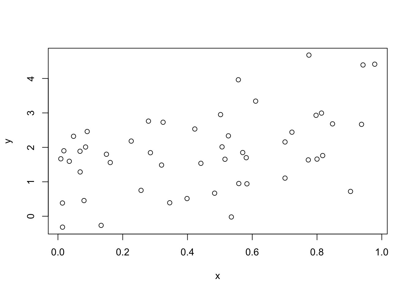
In the code above I needed to define the sample size, and model coefficients, and the standard deviation of the errors (sigma). Then I generated a range of x values from a uniform distribution between 0 and 1 (however you could change the range or even the distribution). Then to generate values of y, I account for the non-random component of y b_0 + b_1 * x and add to this the random component drawn from a normal distribution with mean 0 and standard deviation equal to sigma. The important thing here is that the size of the vector of random component needs to match the fixed part, which I accomplished by using drawing N values of x and N values from the normal distribution.
You can use this basic structure to generate many types of linear models. The advantage of simulations compared to the real world is that we know the true model that generated the data, and therefor we can check if our statistical inferences are correct. For example, the definition of confidence intervals is that we expect them to contain the true parameter about 95 percent of the time. With simulations, we can actually see if this is correct or not by repeating the simulations above many times, and checking how often the estimate 95% CI contain the true parameter (e.g. \(b_1\) in the example above.)
Importantly, we can also use simulations to create cases where we know assumptions of our model are violated. For example, we can generate datasets where the errors are not normally distributed, or where variance increase systematically with either the dependent or independent variable and then check whether our statistical inferences are robust to these violations.
3.9 What you need to know
1. What a sampling distribution is and how it relates to standard errors: If we repeat a study many times, we would get a distribution of parameter estimates. The standard deviations of these distributions is the standard error of a parameter estimate. Although we generally don’t repeat our studies many times, we can estimate standard errors for parameters from our sample. In general, standard errors increase in proportion to standard deviation of the errors/residuals, and decrease in proportion to the square root of sample size.
2. Be able to interpret standard errors and understand what they imply about the likely ranges of parameter values.
3. You should be able to understand the relationship between dnorm(), pnorm(), and qnorm(), and how to use them.
4. You should have an intuitive understanding of confidence intervals, how it relates to the area under the normal pdf, and be able to use the quick and dirty 2 SE value to calculate them.