Chapter 12 Model analysis with deBif

In the computer labs we will use an R package called deBif that is specifically designed for the numerical analysis of (systems of) ordinary differential equations (ODEs). The package includes two basic functions, called deBif::phaseplane() and deBif::bifurcation(). The function phaseplane() allows for the numerical integration of (systems of) ODEs and for analysis of these ODEs in their phaseplane. In addition to numerical integration of ODEs the function bifurcation() allows for numerical bifurcation analysis of ODEs as a function of a single bifurcation parameter and for computing bifurcation curves as a function of two free parameters.

12.1 Installation of `deBif`

12.1.1 Installation of `deBif` as binary package from CRAN

To use the deBif package you will need a recent version of R as well as Rstudio and a range of additional R packages that are required.

Here are the necessary steps for the installation of R and Rstudio:

The version of Rstudio you use is not as critical as the version of R. Updating Rstudio is however easy and can be done via the following link:

https://rstudio.com/products/rstudio/download/
The version of R you are using is critical. When you start up Rstudio you will see a welcome message in the pane of Rstudio that is called Console. The welcome message shows the version of R that you have installed. The version has to be at least 4.0. The package that we are going to use has been tested to work under R version 4.2.2 on Mac OS and version 4.0.3 on Windows. If you need to update your R installation, visit the following link:

https://cran.r-project.org

The deBif package is available on CRAN (The Comprehensive R Archive Network). Therefore, once you have R and Rstudio installed you can most easily install deBif by choosing Tools->Install Packages in Rstudio and typing in the name. This will install deBif as well as the R packages that are needed to run the programs.

Once you have everything installed, you can load and test the package with the following 2 statements:

library(deBif)
deBifExample("rosenzweig")

12.1.2 Installation the most recent version of `deBif`

In case installation from CRAN fails or you want to install the most recent version of deBif from GitHub, the package has to be compiled and your R has to be tailored for that. Make sure that the appropriate versions of R and Rstudio have been installed as described in the previous section.

If you are working on Windows you will have to install both the base part of R as well as Rtools, which is needed to install packages that require compilation (you will need this for the package deBif). You can install Rtools from

https://cran.r-project.org/bin/windows/Rtools/

The recommended version of Rtools at the moment is Rtools42. The installation of Rtools takes some time.
Once you have the appropriate versions of Rstudio and R you first have to install the package devtools. You can do this by executing the command:
```
install.packages("devtools", type = "binary")
```
This command will download and install a range of R packages that are required by the devtools package, but should finish successfully. If you are asked to install these new packages, answer ‘yes’. In case you are asked to install from source and compile (this should not happen with the argument type = "binary"), answer ‘no’ to just install the compiled packages.
Once the package devtools is installed, the package deBif can be installed with the following command:
```
devtools::install_github("amderoos/deBif")
```
This will once again install additional packages that are required by the program. On my Windows my machine, after installing a new version of both Rstudio and R the devtools::install_github command failed with a message that ‘Git’ was not installed on my system. This was however solved by installing the package git2r, either via Tools -> Install packages or by executing the command install.packages("git2r", type = "binary").
Once you have everything installed, you can load and test the package with the following 2 statements:
```
library(deBif)
deBifExample("rosenzweig")
```

12.2 Model implementation

Before you begin with one of the following computer labs, first read how a system of ODEs has to be implemented in R to allow its analysis with either phaseplane() or bifurcation(). These two functions work with the same implementation of a system of ODEs. Section 1 of the manual for the deBif package describes in more detail how to implement the ODEs and how to use the functions phaseplane() and bifurcation(), although the graphical interface of these two function is rather intuitive and self-explanatory. You access the manual by executing in Rstudio the command:

deBifHelp()

The implementation of a model is identical to the implementation used in the package deSolve for systems of ODEs. The model implementation has 3 elements: a vector of state variables, a vector of parameters and the specification of the right-hand side of the ODEs. Both the vector of state variables and the vector of parameters, should consist of named vector elements only. The right-hand sides of the ODEs have to be specified in a R function with a name that you can choose yourself.

As an example, consider the logistic growth model:

\[\begin{align*} \dfrac{dN}{dt}&=\;r N \left(1- \dfrac{N}{K}\right) \end{align*}\]

with variable \(N\) representing the population density. The parameters in this model are the per-capita growth rate \(r\) and its carrying capacity \(K\).

To implement this model first a named vector of values for the state variables has to be defined:

state <- c(N = 0.01)

and similarly a named vector of default values for the parameters:

parms <- c(r = 0.1, K = 10.0)

The named elements of the state variable vector and the parameter vector can now be used in the function that described the right-hand side of the ODEs:

logistic <- function(t, state, parms) {
  with(as.list(c(state,parms)), {

    dNdt = r*N*(1 - N/K)

    return(list(c(dNdt)))
  })
}

To carry out bifurcation analysis of the logistic growth model implemented above an R script can be created with the following content:

# The initial state of the system has to be 
# specified as a named vector of state values.
state <- c(N = 0.01)

# Parameters has to be specified as a named vector of parameters.
parms <- c(r = 0.1, K = 1.0)

# The model has to be specified as a function that returns
# the derivatives as a list. You can adapt the body below
# to represent your model
logistic <- function(t, state, parms) {
  with(as.list(c(state,parms)), {

    dNdt = r*N*(1 - N/K)

    # The order of the derivatives in the returned list has to be
    # identical to the order of the state variables contained in
    # the argument `state`
    return(list(c(dNdt)))
  })
}

bifurcation(logistic, state, parms)

For more details see Section 1 of the manual for the deBif package.

12.3 Computer practical 1: The spruce-budworm (Choristoneura fumiferana)

The spruce budworm (Choristoneura fumiferana) is a moth that inhabits northern American pine forests. Normally, the density of these moths is not very high, and their impact upon the forest is small. However, approximately once every 40 years, their density increases explosively, and entire forests are picked clean of needles in a very short time span. Obviously, this has severe negative effects on local timber production. The major predators of these budworms are birds, and at high densities budworms make up a major part of the birds diet. The budworms themselves eat the newly emerging needles of pine and spruce trees.

The following model, in terms of a single ordinary differential equation (ODE), has been proposed for the growth of the budworm population in the absence of any bird predators. \[ \dfrac{dN}{dt}\;=\;r\,N\,\left(1\:-\:\dfrac{N}{K}\right) \] Here \(N\) stands for the abundance of the budworm population, \(r\) is the intrinsic growth rate (per day), and \(K\) is the carrying capacity of the budworm population. This is the familiar logistic growth equation that describes the growth of most self-limiting populations. We are interested in describing the qualitative behavior of the budworm population in northern American pine forests and wish to show how bird predation may play a role in the regular outbreaks of budworms. For the sake of simplicity, we will start with this simplest of models.

Implement the model as explained above (see for more details the deBif manual). Take \(r=0.1\) and \(K=10\) and \(N=0.1\) to start with. Use phaseplane() to investigate the properties of the right-hand side of the differential equation for different values of \(r\) and \(K\). In the phaseplane() application the right-hand side of the differential equation can be investigated using the tab sheet Nullclines. Which equilibria can you find? How do they change as a function of \(K\) and \(r\)?
Now switch to bifurcation() and compute some time series for different parameter combinations of \(K\) and \(r\). Use this as an exercise to familiarize yourself with bifurcation().
Subsequently, use bifurcation() to construct a graph of the equilibrium as a function of \(K\).

To account for the predation by birds the following modification of the logistic growth model has been proposed, which has been used to explain the outbreaks of budworm population dynamics.

\[ \frac{dN}{dt} \, = \, rN(1-\frac{N}{K})-\frac{EPN^2}{N_0^2 + N^2}\\ \] with \(K = qA\) and \(N_0 = fA\).

Both \(K\) and \(N_0\) now depend on \(A\), which is the leaf (or needle) density of the forest. Of course, in reality \(A\) is not a constant. But the dynamics of the forest are on such a slow timescale compared to the dynamics of the budworms, that we treat it as such. \(P\), the density of the predatory birds, is also assumed constant. this is because if budworm density is low, the birds either switch to other prey, or migrate out of the area. Either way, there is no numerical response of birds to changes in budworm density.

A valid parameter setting for this model is: \(A=0.5\), \(q=20\), \(E=0.314\), \(f=0.474\), \(P=0.7\) and \(r=0.1\).

This parameter setting reflects the conditions in North American pine forests.

Use the implementation of the logistic growth equation that you have used for the previous assignments as a basis to implement this variant of the model in R for analysis with phaseplane() and bifurcation().
Use phaseplane() to compute several time series for the default parameter set, while varying the initial value of \(N\). Make sure to study not only high population densities, but also to consider the range \(N=0.0\ldots0.1\).
Repeat this procedure for various values of \(A\) between 0.1 and 5.0. What is the most remarkable feature that you encounter?
Now investigate the right-hand side of the differential equation as a function of \(N\) using phaseplane(). Do this for a number of different values of \(A\) between 0.1 and 5.0. Explain the results you obtained by integration using the changes you observe in the graphs of the right-hand side of the differential equation.
Turn to bifurcation(). Compute a time series and select its final point to start a continuation of the equilibrium as a function of \(A\). Relate your findings of the integrations to the picture you have constructed.
Explain in words the mechanism behind the regular outbreaks of the spruce budworm in North American forests.
One way to prevent outbreaks is to spray the forest with insecticides. Assume that this would make a smaller fraction of the foliage available for consumption by the budworms, i.e. change the value of \(q\). We can obtain insight about the dynamics of the model for various combinations of \(A\) and \(q\) by continuing the limit points (LP) as a function of these two parameters. In bifurcation() use the tab sheet 2 parameter bifurcation with the two parameters on the axes. As initial point now choose one of the limit points that have been computed and continue it.
Interpret the graph you have just constructed. To that end, sketch the bifurcation graphs of the density \(N\) as a function of \(A\) for different values of \(q\). What does the point denoted ``CP’’ represent? What type of structural change occurs at this particular point?
Repeat the limit point continuation for the parameters combination \(A\) and \(P\). \(P\) could be increased by providing more nesting sites for birds. Is this an effective strategy to prevent budworm outbreaks?

12.4 Computer practical 2: A simple molecular switch

Eukaryotic cells replicate and divide in a cyclic process consisting of four distinct phases: in the G1 phase the chromosomes are unreplicated and the cell grows in size; In the S phase copies of chromosomes are generated through DNA synthesis; The G2 phase follows when DNA synthesis is completed and corresponds to a gap phase during which the cell prepares for mitosis. G2 cells are defined by having fully replicated chromosomes that have not yet started the mitotic process. Finally, during the M phase mitosis occurs and the cell divides.

The cell division cycle is not an autonomous oscillator, like a circadian rhythm, but rather a circular sequence of events that must be carried out in a specific order. The order of events is enforced by checkpoints that control progression from one stage of the cell cycle to the next. The transitions can be made only if the prior event is properly accomplished. Cell cycle transitions are irreversible (ratchet-like) because they are implemented by bistable switches in the dynamics of the underlying molecular regulatory network. The irreversible progression through the cell cycle means that S and M phases always occur in strict alternation, separated by gaps—G1 and G2. When functioning properly, the cell cycle moves steadily forward like a ratchet device, not slipping backwards, say, to do two rounds of DNA synthesis without an intermediate mitosis.

In this computer lab we will analyze a simple model for a molecular switch that can serve as a checkpoint controlling transition from one stage to the next. This model is based on the seminal work by John Tyson and Bela Novak (Tyson and Novak 2013) and is representative for the working of the transcription factor E2F for CycE, a protein kinase active in the late G1 phase of the cell cycle. This transcription factor upregulates the expression of its own gene in a fashion shown in the following wiring diagram:

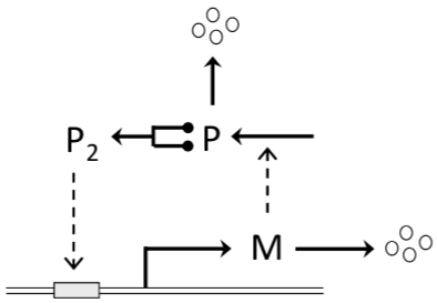
Wiring diagram of a bistable molecular switch (Tyson and Novak 2013). The synthesis of protein P is directed by mRNA indicated with M, which is transcribed from a gene controlled by a promoter (gray box on the double-stranded DNA molecule). The promoter is active when it is bound by dimers (or tetramers) of P.

Figure 12.1: Wiring diagram of a bistable molecular switch (Tyson and Novak 2013). The synthesis of protein P is directed by mRNA indicated with M, which is transcribed from a gene controlled by a promoter (gray box on the double-stranded DNA molecule). The promoter is active when it is bound by dimers (or tetramers) of P.

A simple model for this molecular switch is given by the following 2 ODEs:

\[\begin{align} \dfrac{dM}{dt}&=k_{sm} H(P) − k_{dm} M \tag{12.1} \\ \dfrac{dP}{dt}&=k_{sp} M − k_{dp} P \tag{12.2} \end{align}\] where \(M\) and \(P\) represent the concentration of mRNA and protein, respectively, the constants \(k_{sm}\), \(k_{dm}\), \(k_{sp}\) and \(k_{dp}\) represent the rate constants for synthesis and degradation of mRNA and protein, and \(H(P)\) is the probability that the gene encoding the transcription factor is being actively transcribed. Let’s suppose that this probability equals 1 when the transcription factor is bound to the gene’s promoter, and equals \(\epsilon\) when not bound. Then the function \(H(P)\) is commonly taken to be a Hill function:

\[\begin{equation} \tag{12.3} H(P)=\dfrac{\epsilon K_p^n + P^n}{K_p^n + P^n} \end{equation}\] where \(K_p\) is the equilibrium dissociation constant (units of concentration, say nM) of the transcription factor-promoter complex, and \(n\) is the Hill exponent, \(n = 2\) or 4 depending on whether the transcription factor binds to the promoter as a homodimer or homotetramer. The parameter \(\epsilon\) represents the probability that the gene encoding the transcription factor is being actively transcribed at a protein concentration equal to 0 (\(P=0\)).

Implement the model as explained in the deBif manual. Use as default starting values of the variables \(M=0.5\) and \(P=0.5\). For the parameters use as default values: \(K_p = 1.0\), \(\epsilon = 0.05\), \(n = 2\), \(k_{sm} = 1.0\), \(k_{dm} = 0.6\), \(k_{sp} = 1.0\) and \(k_{dp} = 0.8\).
Use phaseplane() to investigate the dynamics of the model for different initial values of \(M\) and \(P\) between 0.1 and 1.0 for the default parameter values. What stable steady states can you identify?
Also study the dynamics with higher and lower values of \(K_p\). What is the effect of changing \(K_p\) on the stable steady states?
Use the Steady states tab of phaseplane() to study the change in isoclines when varying the value of \(K_p\) and relate this to the dynamics of \(M\) and \(P\) you observed for these \(K_p\) values.
Use the Portrait tab of phaseplane() to study the basin of attraction of the different steady states for different values of \(K_p\). What can you conclude about the basins of attraction?
Use bifurcation() to construct the bifurcation graph of the molecular switch model as function of \(K_p\) for otherwise default parameter values. What is the range of \(K_p\) values for which alternate stable states occur?
Use bifurcation() to construct the dynamic regime graph of the molecular switch model as function of \(K_p\) and \(\epsilon\). For which values of \(K_p\) and \(\epsilon\) are alternate steady states more prominent?
Based on the dynamic regime graph also study the bifurcation graph of the molecular switch model as function of \(K_p\) for a value of \(\epsilon\) for which you expect a qualitatively different graph than for default parameters.
Describe how this simple molecular network can operate as an on/off switch.

The above exercises assumed that the transcription factor \(P\) binds to the promoter as a homodimer and hence \(n = 2\). From here on assume that \(P\) binds as a homotetramer to the promotor and therefore adopt \(n=4\).

Use the Steady states tab of phaseplane() to study the change in isoclines when varying the value of \(K_p\).
Use the Portrait tab of phaseplane() to study the basin of attraction of the different steady states for \(K_p = 1.0\). What can you conclude about the basins of attraction?
Use bifurcation() to construct the bifurcation graph of the molecular switch model as function of \(K_p\) for otherwise default parameter values. What is the range of \(K_p\) values for which alternate stable states occur?
Use bifurcation() to construct the dynamic regime graph of the molecular switch model as function of \(K_p\) and \(\epsilon\). For which values of \(K_p\) and \(\epsilon\) are alternate steady states more prominent?
What can you conclude on the basis of your analysis about the difference in controlling capacity of \(P\) binds as a homodimer or a homotetramer to its promotor?

12.5 Computer practical 3: A juvenile disease model

For this class it will pay off if you install the latest development version of the package deBif using the following two commands:

install.packages("devtools")

devtools::install_github("amderoos/deBif")

If you have the package devtools installed the first of these statement is superfluous and can be skipped.

Notice, however, that this newer version requires that you have version 4.2 or later of R installed as well as updated versions of all packages. The latter can be checked in Rstudio by selecting Tools -> Check for Package Updates....

The main difference of this new version is that it will distinguish between stable and unstable limit cycles when continuing a limit cycle in a bifurcation graph.

For many animal species population growth is not so much limited by reproduction but rather by the development during the juvenile stage, from birth till the onset of reproduction. At the same time animals are facing many diseases that are primarily infecting juvenile rather than adult individuals. In this computer lab we explore the interplay between these two processes, juvenile maturation limiting population growth and juvenile diseases, specifically focusing on the stability of possible equilibrium states and the occurrence of cycles in population abundance.

To model population growth limited by the rate of juvenile maturation we will assume that adults reproduce at a constant per-capita rate \(f\). Juvenile and adult individuals are assumed to experience instantaneous per-capita mortality rates equal to \(\mu_J\) and \(\mu_A\), respectively. Only the per-capita maturation rate of juveniles into adults is assumed to be density dependent and is modeled by:

\[ \dfrac{m}{1 + J^2} \]

Together these assumptions on the life-history rates lead to the following system of ordinary differential equations describing the dynamics of juveniles \(J\) and adults \(A\):

\[ \begin{split} \dfrac{dJ}{dt} &=\;f A - \dfrac{m J}{1 + J^2} - \mu_J J \\[2ex] \dfrac{dA}{dt} &=\;\dfrac{m J}{1 + J^2} - \mu_A A \end{split} \] As default parameters we will adopt \(f = 0.6\) \(m = 20\), \(\mu_J = 0.5\) and \(\mu_A = 0.2\). The parameter \(\mu_A\), representing the mortality rate of adults, will be the main focus of the explorations below.

Plot the total maturation rate of juveniles, \(m J / (1 + J^2)\), as a function of juvenile density to gain insight in the extent of density dependence in maturation. Give a biological interpretation of the shape of the curve and speculate on what biological consequences increases in mortality might have.
Implement the model and use the function phaseplane() to study the isoclines, steady states and the phase portraits with flow fields for different values of \(\mu_A\) ranging from 0.2 till 0.7. Save images of the phaseplanes that qualitatively differ from each other.
Now use the function bifurcation() to study the curves representing steady states of the model as a function of \(\mu_A\) in the range 0.2 to 0.7. If you encounter any Hopf bifurcation points, use these points as starting point to continue the curves representing the limit cycle that originates in these Hopf bifurcation points. Verify the correspondence between the bifurcation diagram you construct here with the results from the previous analysis with the function phaseplane(). Pay special attention to results that seems from a biological perspective counter-intuitive. Tip: If you do not find a branching point (BP), think about what equilibrium state should occur for \(\mu_A=0.7\) and compute the curve for this equilibrium state for decreasing values of \(\mu_A\).
Construct a 2-parameter bifurcation graph as a function of \(\mu_A\) and \(m\).

We will now modify the model to account for a disease that only affects juvenile individuals. The model will therefore be extended with an ordinary differential equation for infected juvenile individuals, which we will refer to as \(J_i\). The per-capita rate at which susceptible juveniles get infected will be assumed to equal \(b J_i\), that means proportional to \(J_i\) with proportionality constant \(b\). The default of \(b\) equals \(b=0.5\). Both susceptible and infected juveniles will contribute to the density dependence in maturation. The per-capita maturation rate of susceptible juveniles will therefore now be modeled with:

\[ \dfrac{m}{1 + (J + J_i)^2} \] The parameter \(m\) has as before a default value of \(m = 20\). Infected juveniles, however, are assumed to develop slower than and hence mature at a per-capita maturation rate

\[ \dfrac{m_i}{1 + (J + J_i)^2} \] in which \(m_i\) has the default value \(m_i = 10\). After maturation infected juveniles are assumed to have no further negative effects of the infection. They hence mature into healthy adults just like the susceptible juveniles.

Write down the system of 3 ordinary differential equations that describe the dynamics of susceptible juveniles, infected juveniles and adults.
Implement the model and use the function bifurcation() to study the curves representing steady states of the model as a function of \(\mu_A\) in the range 0.2 to 0.7. If you encounter any Hopf bifurcation points, use these points as starting point to continue the curves representing the limit cycle that originates in these Hopf bifurcation points.
Use time series simulations of the model dynamics for different values of \(\mu_A\) to gain insight into the dynamics for different ranges of \(\mu_A\), in particular focusing on the persistence of the disease and its effect on the stability of equilibrium states.
What can you conclude about the effect of the disease on the tendency of the population to cycle and about the effect of cycles in population dynamics on the possibility of the disease to persist?

12.6 Computer practical 4: The Paradox of Enrichment and its complications

We will examine the effects of an increase of nutrient input into a lake populated by phytoplankton “prey” (\(P\)) and Daphnia “predators” (\(D\)) feeding on phytoplankton.

\[\begin{eqnarray*} \dfrac{dP}{dt}&=&r\,P\,\left(1\:-\:\dfrac{P}{K}\right)\;-\;f(P)\,D\\[2ex] \dfrac{dD}{dt}&=&\epsilon\,f(P)\,D\:-\:\delta\,D \end{eqnarray*}\]

Phytoplankton grows logistically with growth rate \(r\) and carrying capacity \(K\). We assume that phytoplankton are nutrient limited, i.e. that a linear increase in phosphorous and nitrogen levels translates into a linear increase in the equilibrium levels that phytoplankton can attain if growing on their own (\(K\)). \(f(P)\) is a function determining how many phytoplankton are eaten by Daphnia given an encounter, \(\epsilon\) is the conversion efficiency of phytoplankton to Daphnia biomass, and \(\delta\) is the Daphnia death rate.

Assume that Daphnia attack phytoplankton according to a satiating, type II functional response. At low prey densities Daphnia are limited by the amount of prey they can find while at high prey densities, Daphnia are limited by the time it takes to handle and digest a prey individual. A function describing this is: \[ f(P)\;=\;\dfrac{a\,P}{1\:+\:a\,T_h\,P} \] with \(a\), the attack rate and \(T_h\) the time it takes a predator to attack and digest a prey individual.
Implement the model in R for analysis with phaseplane() and bifurcation(), with parameters \(r=0.2\), \(\epsilon=1\), \(a=0.02\), \(\delta=0.25\), and \(T_h=1\). First examine using phaseplane() the effect of increasing \(K\). What equilibria are possible? Are they stable/unstable? When is coexistence possible? When not? Now examine your findings in bifurcation(). Make several time series with different initial conditions. What is the effect of increasing carrying capacity?
Examine your equilibria as a function of \(K\) in bifurcation().
What is a Hopf bifurcation?
Point out when a Hopf bifurcation occurs in terms of the configuration of your predator/prey isoclines.
What is the “paradox of enrichment”?
Why does the paradox of enrichment occur? (In words or in math).
Construct the Hopf bifurcation boundary as a function of \(K\) and \(\delta\). This boundary separates the parameter combinations for which limit cycles occur from those for which the equilibrium is stable.
Sketch with pen and paper a bifurcation diagram as a function of \(\delta\), based on your \((\delta,K)\)-graph and the bifurcation diagram as a function of \(K\).
Use bifurcation() to locate the existence boundary of Daphnia as a function of \(K\) and \(\delta\).
A challenge: Use a 3D-plot to visualize the limit cycle as a function of \(K\).

Introducing fish predation

The interactions between Daphnia and phytoplankton lead to destabilization with increasing carrying capacity. The objective in this part will be to examine the robustness of those conclusions to predation pressure by fish (\(C\)) on Daphnia. Fish imposed mortality saturates according to a type III functional response. We assume that fish stocks are constant at \(C\).

\[\begin{eqnarray*} \dfrac{dP}{dt}&=&r\,P\,\left(1\:-\:\dfrac{P}{K}\right)\;-\;f(P)\,D\\[2ex] \dfrac{dD}{dt}&=&\epsilon\,f(P)\,D\:-\:d(D) \end{eqnarray*}\]

in which

\[ f(P)\;=\;\dfrac{a\,P}{1\:+\:a\,T_h\,P} \] and

\[ d(D)\;=\;\delta\,D\:+\:C\,\dfrac{D^2}{1\,+\,A_d\,D^2} \] Use parameters \(r=2\), \(\epsilon=0.5\), \(A_d=44.444\), \(C=6.667\), \(a=9.1463\), \(T_h=0.667\), \(\delta=0.1\).

NB: There is no particular order in the suggestions given under the study questions.

Occurrence and stability of equilibria: Start with the qualitative behavior of the model for different levels of productivity (i.e. different values of \(K\), between 0 and 1.0) by studying:
- Isocline configurations in the phase-plane (use phaseplane()).
- Time series starting from different initial conditions (use phaseplane() and/or bifurcation()).
- Bifurcation of equilibria as a function of \(K\).
- Limit cycles (or the minima and maxima of these) as a function of \(K\).
- The global behavior of the model. Make sure you have a picture (mentally or on paper) of the isocline configurations in every different region of \(K\).
How does the bifurcation graph over \(K\) compare to the system without fish predation on Daphnia as analyzed in the preceding steps of this computer lab? Make an explicit comparison of the bifurcation graphs in the two systems and describe the qualitatively different regions.
Effects of predator-induced mortality: Continue with the qualitative behavior of the model for different values of \(C\), by studying:
- Isocline configurations in the phase-plane (use phaseplane()).
- Time series starting from different initial conditions (use phaseplane() and/or bifurcation()).
- Two-parameter bifurcation of all (3 types of) special points found in the bifurcation over \(K\). Deduce from the two-parameter plot a bifurcation graph of the equilibria in the system as a function of \(C\), for different values of \(K\); verify your interpretation with the help of bifurcation().
Biological interpretation: What is the effect of a top-predator on the paradox of enrichment?