Chapter 8 Introduction to R
R is a programming language that is often used for biological data analysis. In the following tutorial, we will discuss some of the basics of working in R. You might already know how to do it, but for those of you who don’t (or for whom it’s been a while) it will probably help with the assignments.
8.1 Installing packages and working directories
Your R session is always stored in a working directory. Importing data sets is much easier when your R session is in the same working directory as the file you want to import. You can check and change the working directory the following ways:
# Find the current working directory
getwd()

# Change the current working directory to a specified location
setwd("C://file/path")
When you work in R (most likely in RStudio), you might have to import new packages. For most packages, you can do so in the following way:
# Install packages (for example 'ggplot2')
install.packages("ggplot2")

# Load package into memory
library(ggplot2)
8.2 Basics of R
8.2.1 Basic data types
R has 5 basic classes, which are important to understand as trying to manipulate the wrong way might lead to frustrating errors. Each data type is used to represent some type of info - numbers, strings, Boolean values, etc.
logical (e.g., TRUE, FALSE)
integer (e.g., 2L, as.integer(3))
numeric (real or decimal) (e.g., 2, 15.5)
complex (e.g., 1 + 4i, 1 + 0i)
character (e.g., “a”, “words”, “names”)
8.2.2 Basic data structures
R has 6 basic data structures, which are the vector, list, matrix, data frame, array and factor. Some of these require that all elements are of the same data type (vectors and matrices) while in others different data types can be combined (lists and data frames).
Vectors
Vectors are the most common basic data structure in R and contain elements that are all of the same type and are single-dimensional. You can create a vector using the c() function. Vectors can contain all data types.
[1] 1 2 3 6 8 20[1] 6Lists
Lists are similar to vectors, but can contain different data types. To create a list, you use the list() function. Lists can contain other data structures as well as data types, even other lists. Lists are one-dimensional but can contain multidimensional data structures.
# Create a list
lst = list(1, c(1,2,3), "hello", FALSE, 5+4i, 5L, matrix(1:9, nrow = 3, ncol = 3))

lst
[[1]]
[1] 1
[[2]]
[1] 1 2 3
[[3]]
[1] "hello"
[[4]]
[1] FALSE
[[5]]
[1] 5+4i
[[6]]
[1] 5
[[7]]
[,1] [,2] [,3]
[1,] 1 4 7
[2,] 2 5 8
[3,] 3 6 9[1] FALSE[1] 3Matrices
Matrices are two-dimensional data structures that contain elements of the same data type. If you make a matrix, the following syntax is used:
matrix(data, nrow, ncol, byrow, dimnames)Where data defines the input values given as a vector, nrow and ncol define the number of rows and columns of the matrix, respectively. byrow tells the matrix to be constructed row-wise if TRUE (and is FALSE by default). dimnames is a list of row/column names.
# Create a matrix containing the numbers 1 to 9, with 3 rows and 3 columns
mat = matrix(c(1:9), nrow = 3, ncol = 3)

mat
[,1] [,2] [,3]
[1,] 1 4 7
[2,] 2 5 8
[3,] 3 6 9[1] 7Data Frames
Data frames are two-dimensional data structures that are essentially lists of same-length vectors. Data frames have the following constraints:
They must have column-names and each row should have a unique name
Each column should have the same number of items
Each column should consist of items of the same type (a vector)
Different columns can have different data types
# Example of a data frame
student_id <- c(1:5)
student_name <- c("raj", "jacob", "iqbal", "shawn", "hitesh")
student_rank <- c("third", "fifth", "second", "fourth", "first")
student.data <- data.frame(student_id , student_name, student_rank)

student.data
student_id student_name student_rank
1 1 raj third
2 2 jacob fifth
3 3 iqbal second
4 4 shawn fourth
5 5 hitesh first[1] 1 2 3 4 5Arrays
Arrays are three-dimensional data structures, consisting of elements on the same data type. They are essentially stacked matrices. If you want to create an array, the following syntax is used:
array(data, dim, dimnames)Where data defines the input values, dim is a vector containing the dimensions of the array and dimnames is a list contains the names of the rows, columns and matrices in the array.
, , 1

     [,1] [,2] [,3]
[1,]    1    3    5
[2,]    2    4    6

, , 2

     [,1] [,2] [,3]
[1,]    7    9   11
[2,]    8   10   12

, , 3

     [,1] [,2] [,3]
[1,]   13   15   17
[2,] 14 16 188.2.3 Comparisons
In R, you can use comparisons to check whether certain conditions are true. When the statement is correct, R returns TRUE and if the statement is not R returns FALSE. The logical operators == and != can be used to compare all kinds of objects. For numeric objects, you can check if they are lesser or greater than other numeric values as well. The following comparison operators exist in R:
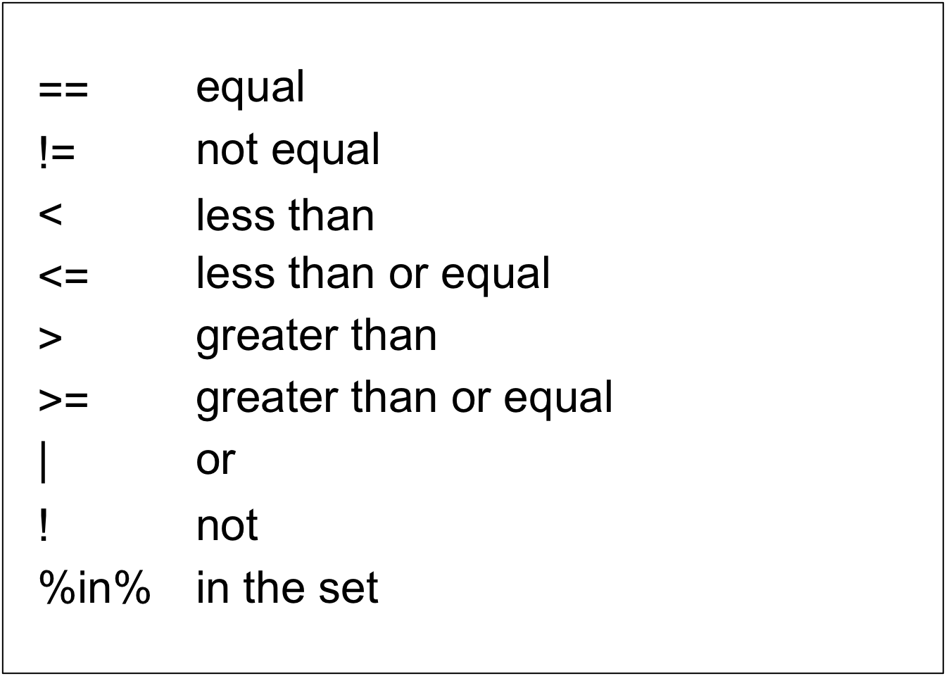
These operations can be combined with & or |. &, meaning “and”, is used when you want to check more than one comparison where ALL comparisons must return TRUE for the entire statement to be TRUE. |, meaning “or”, is used when you want to check more than one comparison where ANY comparison returns TRUE.
[1] TRUE[1] FALSE[1] TRUE[1] TRUE“&” vs “&&” and “\(|\)” vs “\(||\)”
When you want to use “and” in your code, there are options & and &&. The single & compares all elements in a vector and returns a logical vector. The double && only compares the first element, even if it operates on vectors:
[1] FALSE FALSE TRUE FALSE FALSE FALSE[1] FALSE[1] TRUEOne thing to note is that && only works on single logical values, e.g., logical vectors of length 1 (like you would pass into an if condition), but & also works on vectors of length greater than 1. When using with if statements, it is thus better to use && and make sure that both connected elements are single values of TRUE and FALSE.
The same thing goes for | and ||.
Difference between ‘%in%’ and ‘in’
The %in% operator is used to identify if an element belongs to a vector or data frame. The result is a logical value.
# Create values and vector
v1 = 3
v2 = 101
vec = c(1,2,3,4,5,6,7,8)

# Check if v1 is part of the vector
v1 %in% vec
[1] TRUE[1] FALSEDo not mistake %in% with in, which is used in for-loops to run through all the elements in the vector! (See the section about for-loops for an example).
8.2.4 TRUE and FALSE
R uses two logical values, TRUE and FALSE. They should be capitalized and not wrapped into quotes for R to recognize them. 0 corresponds to FALSE, while 1 corresponds TRUE. You can perform calculations using these logical values.
z = c(TRUE, FALSE, TRUE, FALSE, TRUE, FALSE, FALSE, TRUE, FALSE)

# Calculates the number of times TRUE is in list z
sum(z)
[1] 4[1] -4 0 -4 0 -4 0 0 -4 0[1] TRUE[1] FALSE[1] TRUE FALSE TRUE FALSE TRUE FALSE FALSE TRUE FALSE[1] 1 0 1 0 1 0 0 1 0You can easily check which values in a vector meet a certain condition, using logical vectors. These logical vectors can be used to index any vector with the same length.
[1] FALSE FALSE FALSE TRUE TRUE FALSE TRUE TRUE[1] FALSE FALSE FALSE FALSE TRUE FALSE FALSE FALSE[1] 1.5 1.6 1.2 3.08.2.5 seq() and rep()
When creating a vector, you can do so by typing in all your values by hand, using c(value1, value2, etc), but if your vector is very large this becomes very annoying. When your vector consists of a sequence with constant steps between the values, you can use seq(from, to, by). When you want to make a vector consisting of the same value repeatedly, you can use rep(value, times).
[1] 1 2 3 4 5 6 7 8 9 10 [1] 1.0 1.5 2.0 2.5 3.0 3.5 4.0 4.5 5.0 5.5 6.0[1] 5 5 5 5 5 5 58.3 If-statements
You use if statements when you only want to perform an action if certain conditions are true. The syntax of the if statement is:
if (condition) {
do something
}
If the condition is TRUE, the statement gets executed. But if it’s FALSE, nothing happens. The condition can be a logical or numeric vector, but only the first element will be checked. When the vector is numeric, only zero is taken as FALSE, the rest is TRUE.
The if...else statement has an additional action if the condition is FALSE. It is essentially the same as the if statement if you would state to do nothing when the condition is FALSE. The syntax of the if...else statement is shown below (note: the else must be in the same line as the closing braces of the if statement):
if (condition) {
do something
} else {
do something else
}
You could make a ladder of statements when there are more than two options. The syntax you would use in this case is:
if (condition1) {
do something
} else if (condition2) {
perform action 2
} else if (condition3) {
perform action 3
} else {
perform action 4
}
To recap:
The essential characteristic of the
ifstatement is that it helps us create a branching path in our code.Both the
ifand theelsekeywords in R are followed by curly brackets { }, which define code blocks.R does not run both, and it uses the comparison operator to decide which code block to run.
8.4 Loops
Programming loops are nothing more than an automatic version of a multi-step process in which you group the steps to be repeated, and perform them multiple times with only a few instructions.
There are two types of loops in programming. The first type consists of loops that execute for a prescribed number for times, controlled by a counter or index. These loops are for-loops. The second type consists of loops that are based on the verification of a logical condition. This condition is checked at the start or the end of the loop. These loops are while or repeat loops, respectively.
8.4.1 For-loops
for-loops specify the number of times a certain action needs to be performed. For example, if you want to perform an action for all values in a vector, using a for-loop saves you a lot of time. for-loops have the following general code:
for (every item in vector) {
    do something
    }
You can define a vector beforehand and use the specific values in the vector as ‘item’ (i).
[1] 0.1
[1] 0.2
[1] 0.3
[1] 0.4
[1] 0.5
[1] 0.6
[1] 0.7
[1] 0.8
When you need the ‘item’ to refer to the index of the values in stead of the real values (for example, when you want to use different data sets in one for-loop or you want to store the output in a new vector), you can define the for-loop-vector using ‘for (i in start value : end value)’, as is done below:
# Create a vector filled with random normal values
u1 = rnorm(n = 8)

# Initialize the vector containing the squared values
usq = 0

# Calculate squared number for all values in u1
for(i in 1:length(u1)) {
  # i-th element of `u1` squared into `i`-th position of `usq`
  usq[i] = u1[i] * u1[i]
  print(usq[i])
}
[1] 7.241391
[1] 0.3578144
[1] 2.596496
[1] 0.1913024
[1] 1.829583
[1] 0.2214347
[1] 0.2211333
[1] 0.1570606[1] 7.2413906 0.3578144 2.5964963 0.1913024 1.8295825 0.2214347 0.2211333 0.1570606Tip: when you get overwhelmed by all the loops, you can use the print() statement to see all the steps in the loop. ‘print(i)’ helps to make sense of which iteration has which result.
Nested for-loops
Nested for loops are loops that contain other loops in their ‘do something’-section. This comes in handy when you work with data sets and matrices, as they need two indices: one for their rows and one for their columns. An example of a nested for loop is shown below (remember that indexing is done as data[row, column]):
# Create a 30 x 30 matrix (of 30 rows and 30 columns)
mymat = matrix(nrow=10, ncol=10)

# For each row and each column, assign values based on position
for (i in 1:nrow(mymat)) {
  for (j in 1:ncol(mymat)) {
    mymat[i,j] = i*j
  }
}

# Show the matrix
mymat
[,1] [,2] [,3] [,4] [,5] [,6] [,7] [,8] [,9] [,10]
[1,] 1 2 3 4 5 6 7 8 9 10
[2,] 2 4 6 8 10 12 14 16 18 20
[3,] 3 6 9 12 15 18 21 24 27 30
[4,] 4 8 12 16 20 24 28 32 36 40
[5,] 5 10 15 20 25 30 35 40 45 50
[6,] 6 12 18 24 30 36 42 48 54 60
[7,] 7 14 21 28 35 42 49 56 63 70
[8,] 8 16 24 32 40 48 56 64 72 80
[9,] 9 18 27 36 45 54 63 72 81 90
[10,] 10 20 30 40 50 60 70 80 90 100Note: Remember that every for-loop needs its own set of curly braces, each with its own block and governed by its own index.
8.4.2 Alternative loops
Sometimes, for-loops are not the best option, when you don’t know or control the number of iterations, for instance. For example, when you need to count the number of clicks on a web page within a specified number of days or other unpredictable events. In these cased, you can use a while- or repeat-loop.
While loops
while-loops often make use of a comparison between a control variable and a value, checking if the value is greater than the control variable, for instance. This check results in a logical response, either TRUE or FALSE. When the result is FALSE, the block of code is not executed and the program will continue with the code below the loop. If the result of the check is TRUE, the block of code gets executed. while-loops only stop running when the result of the check changes from TRUE to FALSE, so updating the control variable in the loop or adding a increment to a counter is needed for the loop to ever stop running. Note that the code will never run if the result is FALSE at the first check. An example of the while-loop is shown below.
[1] 0.2
[1] 0.4
[1] 0.6
[1] 0.8
[1] 1
Repeat loops and break
The repeat-loop is similar to the while-loop, but its block of code is executed at least once, no matter the result of the condition. You could call this loop ‘repeat until’, as it is executed until the condition changes and the loop ‘breaks’. When R encounters a break, it leaves the loop and continues with the code below it (if any). If the break is part of a nested loop, it will only exit the loop it is a part of. An example of the repeat-loop is shown below.
[1] 1
[1] 2
[1] 3
[1] 4
[1] 5
Note: be careful to specify the termination-condition when you use the repeat- loop, as you might end up in an infinite loop otherwise!
8.5 The runif() function
The runif() function generates random deviates of the uniform distribution (and has nothing to do with if-statements). runif() needs an input ‘n’, ‘min’ and ‘max’, which correspond to the number of values between the ‘min’ and ‘max’ values. It can be used to produce random numbers, and has fractional numbers as output.
The runif() function is useful when simulating probability problems, as show below.
# Make a vector of probabilities
x = runif(10, min=0, max=1)
# Check for every value in the vector x if it exceeds 0.6. If so, print that value
for (i in 1:length(x)) {
    if (x[i] > 0.6) {
    print(x[i])
    }
}
[1] 0.7431598
[1] 0.6412899
[1] 0.890269
[1] 0.7646008
[1] 0.83478
[1] 0.9935257
[1] 0.90990278.6 The sample() function
The sample() function draws a random sample of a specified size from a population of values, either with replacement or without replacement. The syntax of the sample() function is as follows:
sample(x, size, replace, prob)Here x is a vector of values. You can use for example the range (1:10) for x if you want to draw a random sample from the numbers 1 to 10. size specifies how many values are to be drawn. replace can either take the value TRUE or FALSE depending on whether you want to sample with or without replacement. The argument replace is optional and takes as default value FALSE. Note, however, that if you sample without replacement the maximum number of items that can be drawn equals the length of the first argument x. Finally, the argument prob can be used to specify what the probability is to draw each of the elements of the vector x. This is also an optional argument, the default value is that each of the the elements in x has the same probability to be drawn.
The sample() function is useful when simulating chance processes. For example, we can simulate the process of tossing a coin 100 times with a single call to sample():
# Possible outcomes are head (0) or tails (1)
values = c(0, 1)

# Toss a coin 100 times
outcomes = sample(values, 100, replace = TRUE)

# How many times did you throw tails?
sum(outcomes)
[1] 468.7 Data Frames and plotting data
8.7.1 Import data frames
When you want to import a (.csv) data frame, you can do so using the following code. This is easiest when your working directory contains the file you want to import.
# Read specified .csv file
df = read.csv("filename.csv")

# You can write in a .csv file too
write.csv(df, "filename.csv")
8.7.2 plot()-function
The simplest function functions to plot your data is the plot function. It allows you to create a plot based on two vectors (of the same length), a data frame, a matrix or other objects. The function has different arguments you can specify, which can be found when you run ?plot.
# Generate data
x = seq(0, 10, by=0.1)
y = sin(x)

# Plot the data (without specifying anything)
plot(x, y)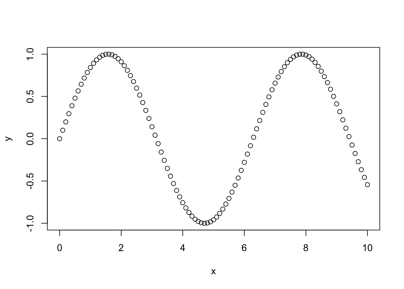
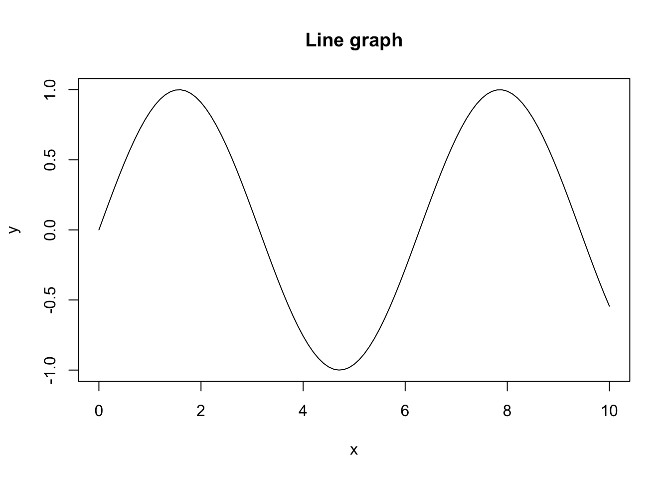
abline(), lines() and points()
When you want to add an additional line to a graph made using plot(), you can so using either abline() or lines(). abline() creates a straight line using the intercept and the slope, while lines() uses a set of vectors to construct a line. points() also uses a set of vectors, but plots them as points rather than a line. Note that all require you use plot() first, as they cannot produce a plot on their own. An example is shown below (check the different style options such as lwd (‘line width’), col (‘color’), lty (‘line type’) and pch (‘plotting symbols’).
# Create some vectors
x = 1:10
y1 = x * x
y2 = 2 * y1

# Create plot of first line
plot(x, y1, type="b", col="red", xlab="x", ylab="y", lwd=2)

# Add second line (as well as points)
lines(x, y2, type="l", col="blue", lty=2, lwd=2)
points(x, y2, col="black", pch=15, lwd=3)

# Add a straight line specifying the intercept and slope
abline(3,4, col="green", lwd=3)

# Add a legend to the plot
legend("topleft", legend=c("plot()", "lines()", "points()", "abline()"),
col = c("red", "blue", "black", "green"), lty= 1:2, cex=0.8) 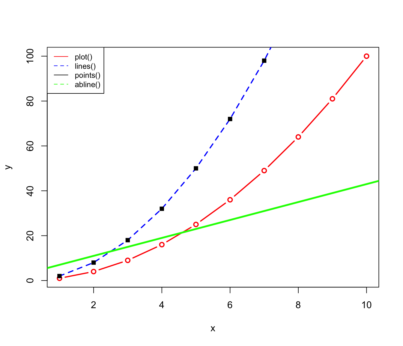
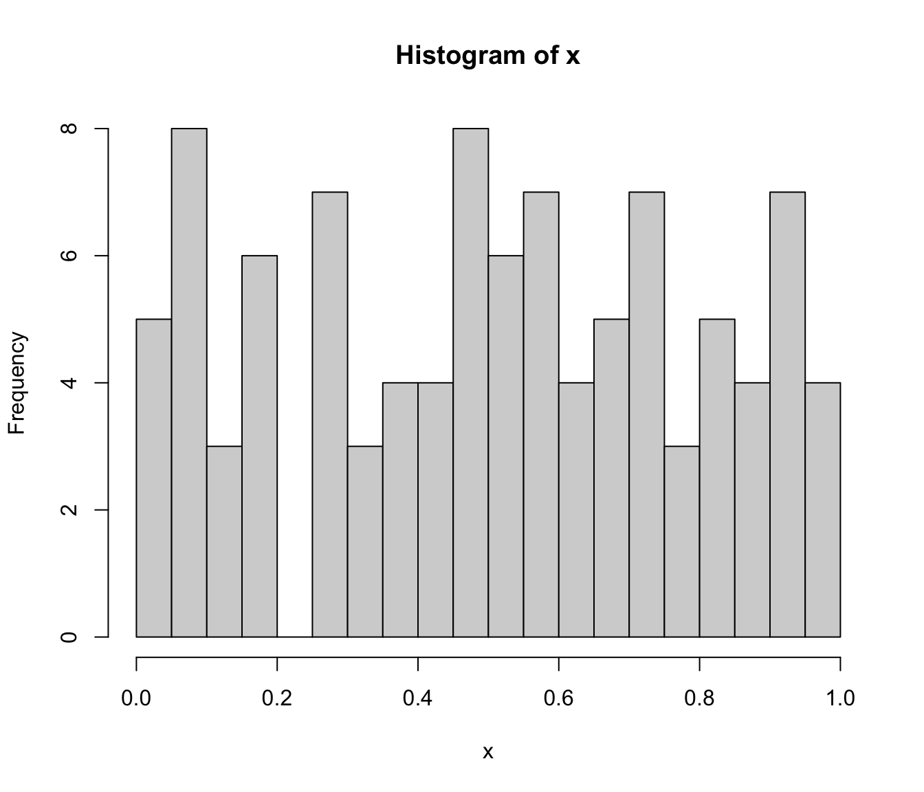
8.7.3 hist() function
The hist() function can be used to create and plot a histogram of results. The syntax of the hist() function is:
hist(x, breaks, freq, right, .....)The 3 dots at the end of this statement means that there are more arguments that you can add, but that these are optional. For a full description of these optional arguments check out the help page on the hist() function using ?hist
The first argument x of the hist() function is a vector of values that has to be sorted into bins. The arguments ‘breaks’ determines the bins. This argument break can be one of the following types:
a single number giving the number of cells for the histogram,
a vector giving the breakpoints between histogram cells,
(More types of arguments are allowed for breaks but they are not so relevant for our purposes. See the help page ?hist if you are interested).
The argument freq should be specified either TRUE or FALSE. If freq is TRUE the number of values in each bin is plotted, otherwise the fraction of all values in each bin is plotted. The default value of freq is TRUE.
The argument right should also be specified either TRUE or FALSE. If right is TRUE then a value a value in x that is exactly equal to right-most boundary of a bin is included in the bin (the histogram cells are right-closed (left open) intervals). The default value of freq is TRUE.
8.7.4 ggplot2()
For more complex kinds of data, for example when you want to compare the data from different groups, it is easier to use ggplot() when plotting your data. ggplot() has many options, which we will not discuss here, but we will give you a short introduction with some examples.
The main difference between ggplot and basic plotting is that ggplot works with data frames and not individual vectors. When using ggplot, you first have to specify which data frame you’re plotting. When your data frame consists of more than two columns (which is usually the case), you have to specify which columns to plot. This can be done the following way:
  Sepal.Length Sepal.Width Petal.Length Petal.Width Species
1          5.1         3.5          1.4         0.2  setosa
2          4.9         3.0          1.4         0.2  setosa
3          4.7         3.2          1.3         0.2  setosa
4          4.6         3.1          1.5         0.2  setosa
5          5.0         3.6          1.4         0.2  setosa
6          5.4         3.9          1.7         0.4  setosa
# Initiate plot (this does not show any data plotted, ggplot wants that specified)
ggplot(iris, aes(x=Species, y=Petal.Length))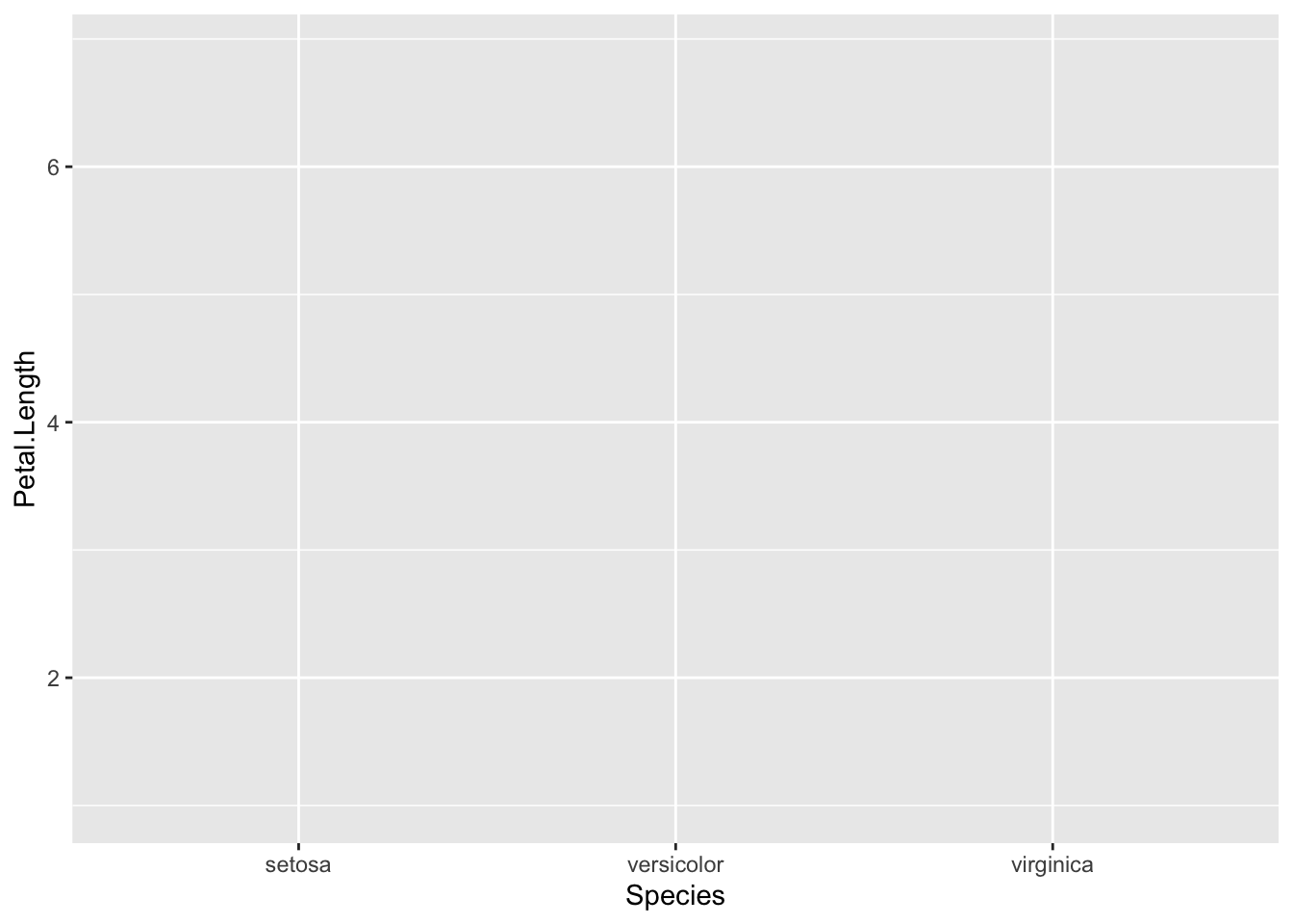
# To specify the type of plot, you need to use 'geom_...'
ggplot(iris, aes(x=Species, y=Petal.Length)) + geom_jitter(aes(color=Species))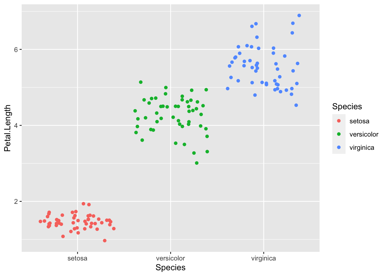
# Using ggplot you can easily add new graphs to the plot
f = ggplot(iris)
g = f + geom_smooth(aes(x=Sepal.Length, y=Sepal.Width, color=Species))
g + geom_point(aes(x=Sepal.Length, y=Sepal.Width, color=Species))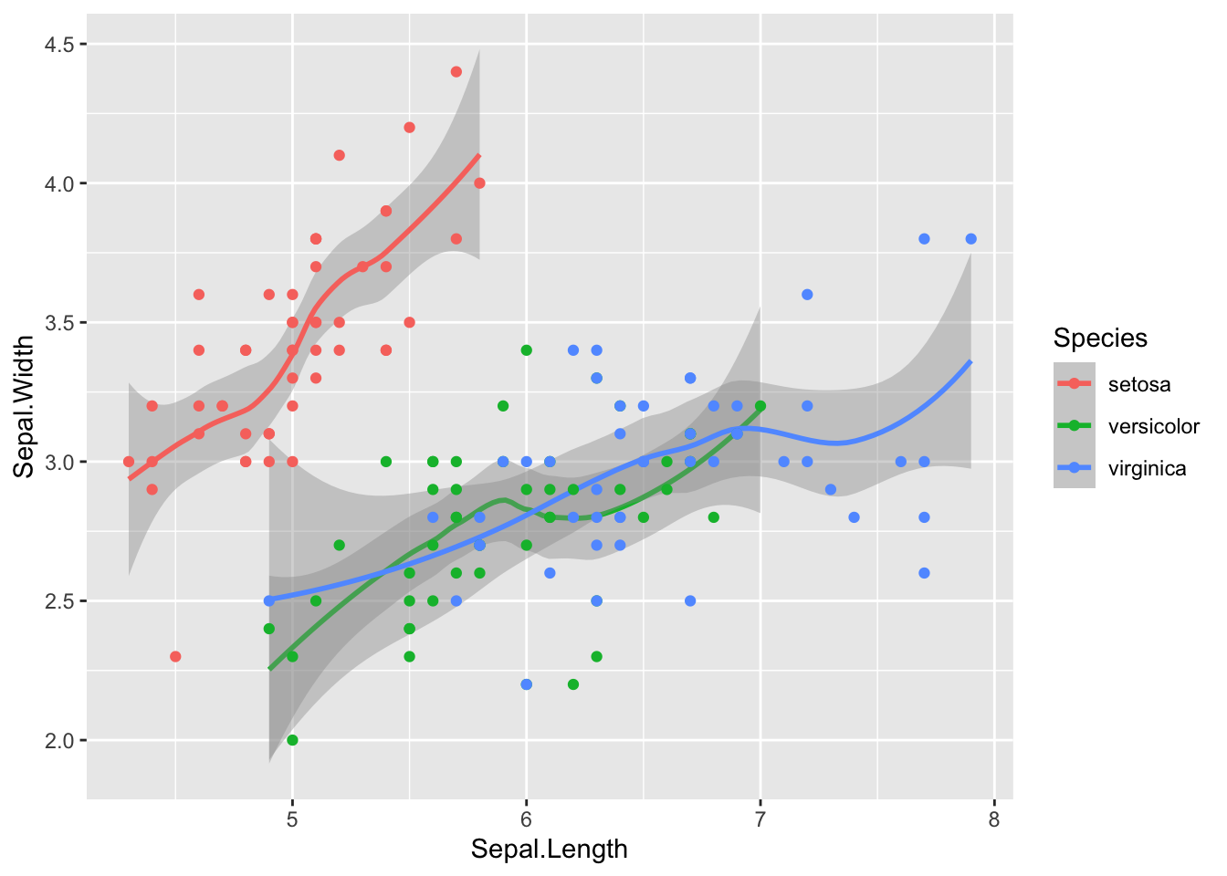
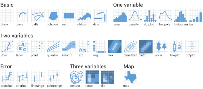
In the aes() argument, you can specify your preferred X- and Y-axis, colour, size, shape and other aesthetic options. If you want to have the color, size etc fixed you need to specify it outside the aes(). Using geom you specify the type of plot you want. There are many options, which are shown in the figure below.
8.8 Exercises
8.8.1 Exercise 1
a. Use the sample() function to simulate an experiment in which you throw a six-sided dice 20 times.
b. Use the hist() function to plot a histogram of the results. How do the results compare with your expectation of the outcome of throwing a dice?
c. Repeat the above steps for throwing the dice 100 and 1000 times.
8.8.2 Exercise 2
a. Create a vector of the values 1 to 10, with steps of 0.5.
b. Using a for-loop randomly draw 20 “grades” from that vector and store them in a new vector. Tip: Use sampling with replacement!
c. For every value in the newly created vector, check if it is higher than or equal to 5.5, and store the result as “PASS” in a newly created vector. If the value is below 5.5, store “FAIL” to that vector.
d. Count the number of people that passed the course (tip: check out the “length”- and “which”-function).
8.8.3 Exercise 3
a. Import the built-in ‘diamonds’ data set and check its content (which is only available after loading the ggplot2 package).
b. How many variables does the data set contain?
c. Create a scatter plot of the carat versus the price, where you also check the influence of the clarity.
d. Change the opacity of the points using the ‘alpha’-function and add a smoothing trend to the plot.
e. Using ggplot, create a histogram of the carats where you check the influence of the cut.
f. Change the x limit to only see the carats between 0 and 2. Change the opacity of the bars as well.
8.8.4 Exercise 4
a. Create a vector containing 20 random numbers.
b. Use a repeat loop to print 10 sampled numbers from that vector. The loop should stop after 10 iterations.
Good luck with the assignments, and remember: when you don’t know how to do something, google can help a lot! You should think about what you want to do specifically, and most of the time you can find the way to do it on Stack Overflow or another forum.
8.9 Sources used (and to check out if you want more information)
Datacamp (https://www.datacamp.com/tracks/data-scientist-with-r)
Codeacademy (https://www.codecademy.com/learn/paths/analyze-data-with-r)
Datamentor (https://www.datamentor.io/r-programming/)
YaRrr! The Pirates Guide to R (https://bookdown.org/ndphillips/YaRrr/)
Dataquest (https://www.dataquest.io/path/data-analyst-r/)
R-Statistics (http://r-statistics.co/)
Ggplot2 (https://ggplot2.tidyverse.org/reference/)
Techvidvan (https://techvidvan.com/tutorials/r-tutorial/)
DataScience Made Simple (https://www.datasciencemadesimple.com/r-tutorial-2/)
RaukR (https://nbisweden.github.io/RaukR-2019/ggplot/presentation/ggplot_presentation.html#1)