Chapter 5 Simulation methods
Previously you might have encountered various types of statistical methods to test hypothesis, such as the \(t\)-test the Chi-squared test. Or you might have learned a formula to compute the confidence interval of particular statistics such as the mean or the median. Such methods are part of analytical statistics, the branch of statistics that heavily relies on analytical expressions to compute, for example, test statistics, standard errors and confidence intervals. These analytical expressions are, however, only valid as long as the assumptions on which they are based are satisfied. For example, a common assumption in analytical statistics is that errors are independent and normally distributed. Whether or not such assumptions are satisfied in particular applications of analytical statistics is often unclear or even doubtful.
Luckily, with the rise in computational power has come the possibility to address many of the problems in applied statistics using an approach, referred to as Monte Carlo simulation, that does not require making the assumptions underlying analytical statistics. The concept of Monte Carlo simulation was developed by the mathematicians Stan Ulam and Nicholas Metropolis. During World War II Ulam and Metropolis were part of the Manhattan Project, the purpose of which was to develop an atomic weapon for the US. One question they had to solve was what the average distance is that a neutron would travel in a substance before it collided with an atomic nucleus. Faced with the situation that this question could not be answered using standard mathematics, Ulam realized that he could use simulations with random numbers to compute the average distance traveled. Just like in a casino game such as a roulette wheel, in such simulations numbers are generated at random and to estimate the probability of a specific outcome, one could play the game many, many times. The story goes that the technique is named after the Monte Carlo casino in Monaco, where Ulam’s uncle used to gamble.
Nowadays Monte Carlo simulation techniques, or simulation techniques for short, are pivotal in many statistical studies. Simulation approaches can be used for different purposes:
To estimate the accuracy or precision of sample statistics
To perform significance tests
To validate models by using random subsets of a data set
To analyse processes, for example to evaluate a particular experimental design or to estimate parameters
All these approaches have a common theme: a particular process is simulated repeatedly very many times, every time with a new set of random numbers or a new random selection of a particular data set. These many repetitions provide a distribution of different outcomes, much like sampling a particular population many times provides a distribution of outcomes. The distribution of the simulation outcomes can be exploited to test hypothesis or compute confidence intervals.
Simulation methods in statistics encompass a suite of different approaches, each with their own names:
Bootstrapping and Jackknifing: Bootstrapping is used to estimate the sampling distribution of a particular estimator by sampling with replacement from the original sample. This procedure allows for the estimation of standard errors and confidence intervals of a population parameter like a mean, median, or regression coefficient. Jackknifing is similar to bootstrapping and is used to estimate the bias and standard error (variance) of a statistic. The basic idea behind the jackknifing is to systematically recompute the estimate of a particular statistic (such as mean or median), leaving out one or more observations at a time from the sampled data set. Given a sample of size \(n\), a distribution of a particular statistic can for example be created from all sub-samples of size \(n-1\) obtained by omitting one observation. This new set of replicates of the statistic provides an estimate of the bias and the variance of the statistic.
Randomization or permutation tests: These are methods used for hypothesis testing. For example, to test the significance of an observed statistic, such as a mean difference between 2 groups, the data is randomly shuffled and the statistic is computed anew for the shuffled data. Comparison of the originally observed value of the statistic with the distribution after reshuffling provides a measure of the likelihood that the observed value is significant or could be the outcome of a random process.
Cross-validation: Cross-validation is a statistical method for validating a predictive model. Given a data set, a model is fit to only part of the data (the so-called training data). The fitted model is subsequently used to predict the other part of the data set that was not used for fitting the model (the validation set). An overall measure of the prediction accuracy of the model can then be obtained from the fit of the model to the validation data.
Monte Carlo methods: Monte Carlo methods, or Monte Carlo experiments, are used to repeatedly simulate a particular process, each time with different random values, to arrive at a distribution of possible outcomes of the process.
In the following we will discuss bootstrapping, hypothesis testing through randomization and Monte Carlo process simulation. However, before doing so and because all the methods rely on generating random numbers, we will first discuss the pseudo-randomness of random numbers.
5.1 Random numbers and how to generate them
Random numbers are crucial for any simulation method, but unfortunately true random numbers can only be generated by a physical process, such as throwing a dice or flipping a coin. The best a computer can do is to generate a sequence of pseudo-random numbers, which are not random at all. In fact, the random numbers that can be generated by a computer program, whether it is R or any other program, are produced by an algorithm that necessarily repeats after a specific number of times. Different types of algorithms exist to generate pseudo-random numbers and R implements at least 7 different options, which you can explore by typing the command ?Random. The default random number generator that R uses us called the Mersenne-Twister, which method repeats after exactly \(2^{19937}-1\) times.
In R the function runif(n) uses the selected random number generator to produces \(n\) different values between 0 and 1 (additional arguments min and max) can be supplied to the runif() function to change the range from which the values are selected). For example:
[1] 0.25699945 0.63990908 0.50690479 0.96627805 0.67166028 0.08302234generates 6 values between 0 and 1 that at first sight look pretty random. The sequence is moreover hard to predict. Repeating the same call illustrates the randomness
[1] 0.8551046 0.4393758 0.5203980 0.9603904 0.5464044 0.5481606and yields an entirely different sequence of 6 random values between 0 and 1.
However, the randomness is elusive, because the sequence of values that is generated is uniquely determined by the seed value of the random number generator. This seed value can be set using the function set.seed() in R. Let’s repeat the previous two calls to runif(), while preceding each call with a call to set.seed() with the same value:
[1] 0.1557190 0.6929711 0.4286529 0.6973091 0.1693208 0.9255609Setting the seed value to 567852 is completely arbitrary here, we could have chosen any other value. But let’s see what happens if we repeat the previous call:
[1] 0.1557190 0.6929711 0.4286529 0.6973091 0.1693208 0.9255609You can see that we obtain exactly the same random number sequence in the two calls, because we set the seed value of the random number generator to the same value. Similarly, if we set the seed value once and generate 2 sequences of 6 random numbers using 2 calls to the runif() function:
[1] 0.1557190 0.6929711 0.4286529 0.6973091 0.1693208 0.9255609[1] 0.06594427 0.03946674 0.84221252 0.74674796 0.49504277 0.12987301we obtain the same sequence of 12 numbers as when the seed value would be set and the runif() is called only once to generate the 12 random numbers all at the same time:
 [1] 0.15571901 0.69297114 0.42865290 0.69730914 0.16932079 0.92556089 0.06594427 0.03946674 0.84221252 0.74674796 0.49504277
[12] 0.12987301
Notice how the last 6 numbers in this last sequence are indeed the same as the numbers generated by the call to runif(6) just before that.
A sequence of random numbers generated by a computer is therefore not random at all, but is uniquely determined by the seed value of the algorithm that generates the sequence of numbers. This unique relationship between the seed value of the random number generator and the sequence of random numbers can be usefully exploited if we want to repeat a particular simulation of a process with exactly the same sequence of random numbers.
5.2 Bootstrapping
Bootstrapping is a simulation-based method to estimate the uncertainty of a particular statistical quantity. In turn, such an estimate of the uncertainty of the statistic can be used to derive a confidence interval for the quantity. As opposed to other approaches to compute confidence intervals, bootstrapping does not make any assumption about the underlying distribution of the statistical quantity.
5.2.1 Confidence interval of the median
To illustrate bootstrapping we focus on computing the median of a particular data set. One of the data sets that is standard available in R is called faithful. This data set contains 272 observations on the duration of the eruptions for the Old Faithful geyser in Yellowstone National Park, Wyoming, USA (see Figure 5.1) and associated with the eruption duration the waiting time till the next eruption.

Figure 5.1: The Old Faithful geyser in Yellowstone National Park, Wyoming, USA.
Here you see the first 8 lines of the data set (accessed by using head(faithful, 8)). The data set contains 2 columns, the first one called eruptions containing the values of the duration of an eruption (in minutes), while the second column called waiting contains the values of the waiting time till the next eruption occurs (also in minutes).
  eruptions waiting
1     3.600      79
2     1.800      54
3     3.333      74
4     2.283      62
5     4.533      85
6     2.883      55
7     4.700      88
8     3.600      85
Let’s focus for the time being on the duration of the eruptions. Here is a histogram of the duration of the eruptions of Old Faithful:
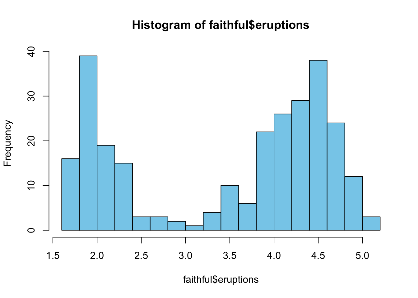
The distribution is clearly bimodal with one peak around a duration of 2 minutes and a second peak around a duration of 4.5 minutes. The median value of the eruptions is 4:
[1] 4Notice that this is the sample median. The question to answer is how we can compute a confidence interval for the median. Given that the distribution is bimodal, methods to compute confidence intervals that are based on an assumption of normally distributed data would obviously be inappropriate. Here bootstrapping is highly valuable and applicable.
The idea of bootstrapping is that we use the data set and treat it like it is a completely unbiased representation of all the eruption durations of Old Faithful. In other words, we adopt the data set not as a sample of a particular population of values but as the entire population of values itself. From this data set we then resample the same number of values as the data set itself contains, but we do this sampling with replacement. The sampling with replacement is here crucial, because we would otherwise end up with a resampled, artificially constructed data set that is identical to the original one. Here are the two statements to construct a new, sampled data set from the Old Faithful data set:
nsample = nrow(faithful)                              # Determine the length of the data set
X = sample(faithful$eruptions, nsample, replace=T)    # Resample with replacement
For the resampled, artificially constructed data set we can again compute the median value, which may or may not be slightly different than the original value. To illustrate that we repeat the resampling and computation of the median 2 times:
[1] 4.075[1] 3.9665[1] 3.833As you can see, the 3 resampled data sets all provide a different estimate for the median value of the duration. We can construct a distribution for these estimates of the median value by repeating the resampling with replacement and the computation of the median value not just 3 times, but very many times. In the code below, an empty vector med_dist is constructed of a length N=10000 and a for loop is used to resample the original data set with replacement 10000 times. The median values of these resampled data set are stored in the elements med_dist[i] of the result vector.
nsample = nrow(faithful)
N = 10000                                               # N determines number of resamplings
med_dist = rep(NA, N)                                   # Create empty vector for results
for(i in 1:N) {
  X = sample(faithful$eruptions, nsample, replace=T)    # Resample with replacement
  med_dist[i] = median(X)                               # Compute median for this sample
  }
The series of median values computed in these iterations (and stored in the variable med_dist) we refer to as the bootstrap median values. Now plot the distribution of these bootstrap median values and compare it with the median value of the original data set:
hist(med_dist, col="orchid")                            # Plot histogram of all results
abline(v=median(faithful$eruptions), col="blue",lwd=4)  # Plot the median of the data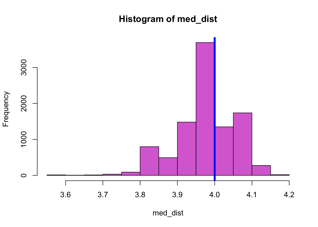
This histogram shows that the bootstrap median values are approximately normally distributed. One approach to calculate a confidence interval for the median is to assume that indeed the bootstrap median values are normally distributed and use the techniques discussed in section 3.6 to estimate the confidence interval. A quick and dirty approach to estimate the confidence interval from the bootstrap median values is then to use the mean of their distribution and subtract or add to that mean value 2 times the standard deviation of their distribution. As also discussed in section 3.6, a more accurate estimate of the confidence interval can be obtained by using the quartile function qnorm() of the normal distribution. More specifically, multiplying the standard deviation of the bootstrap median values by qnorm(0.025) and qnorm(0.975), respectively, and adding the result to the mean of the distribution gives the range of values that contains 95% of the median values that are obtained from the resampled data sets. The results in the following confidence interval for the median value of the eruption duration of Old Faithful:
[1] 3.830590 4.139324One disadvantage of using this approach to estimate a confidence interval is that it requires again an assumption that the bootstrap median values are normally distributed. This type of bootstrap is also referred to as Normal bootstrapping as it depends on this assumption of normality. An alternative approach to calculate a confidence interval from the bootstrap median values is to sort all the bootstrap median values from low to high and then select the element \(0.025 \cdot N\) (= 250 in the example where \(N=10000\)) as lower bound of the confidence interval and the element \(0.975 \cdot N\) (= 9750 in the example where \(N=10000\)) as upper bound of the confidence interval on the grounds that 95% of the computed bootstrap median values fall in between these two limits. This approach to compute the confidence interval is referred to as Percentile bootstrapping because it uses the percentile of bootstrap median values that is below the lower threshold and above the upper threshold as determinant for the confidence interval. The result is the following:
med_dist_sorted = sort(med_dist)
c(med_dist_sorted[0.025 * length(med_dist_sorted)], med_dist_sorted[0.975 * length(med_dist_sorted)])
[1] 3.8330 4.1085As can be seen the confidence interval estimated using Percentile bootstrapping is slightly narrower then the confidence interval estimated using Normal bootstrapping. Percentile bootstrapping is also preferable over Normal bootstrapping as it results in asymmetric confidence intervals. As can be seen from the last displayed results, the lower bound of the confidence interval is 0.167 below the median value computed from the Old Faithful geyser data (median(faithful$eruptions) = 4), while the upper bound is only 0.108 higher than this median.
To carry out Percentile bootstrapping in R it is more easy to use the function quantile() on the unsorted vector of values. This function determines from the values the thresholds that include 95% of all observations if we specify 2.5% and 97.5% as arguments in the following manner:
  2.5%  97.5%
3.8330 4.1085
5.2.2 Confidence interval for other statistics
As stated in the beginning bootstrapping can be used to estimate the confidence interval for any statistic. Consider, for example, the correlation between the duration of an eruption of Old Faithful and the waiting time till the next eruption of the geyser. Plotting these two variables against each other clearly shows that after an eruption that has lasted long, the waiting time till the next eruption is also long, as shown in the following plot:
par(mar = c(6,6,2,1))
plot(faithful, pch = 19, xlab = 'Duration of eruption (min.)', ylab = 'Waiting time (min.)', cex.lab = 1.5, cex.axis = 1.25, yaxt = 'n')
axis(2, las = 2, cex.axis = 1.25)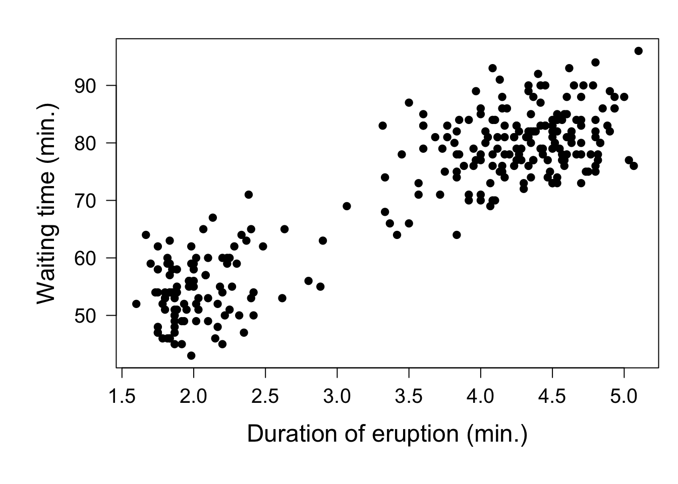
We can now compute the correlation between these two variables using the function cor():
          eruptions   waiting
eruptions 1.0000000 0.9008112
waiting   0.9008112 1.0000000
The result of cor() is a \(2 \times 2\) matrix with correlation coefficients. The diagonal elements of this \(2 \times 2\) matrix equal 1 (implying perfect correlation) since any variable is of course perfectly correlated with itself. The two off-diagonal elements are equal as they both represent the correlation between the duration of an eruption and the waiting time till the next eruption. We can now compute a confidence interval for this correlation coefficient between the duration of an eruption and the waiting time till the next eruption using bootstrapping in much the same way as discussed in the previous subsection. However, because we are dealing here with pairs of data (a pair of a duration and a waiting time), there is a little twist: we have to resample the rows of the data set and keep the pair of duration and waiting time in each row always together. The following code lines first determine the number of rows (observation pairs) in the original data set (variable nsample) and then sample from all the row indices ((1:nsample)) with replacement as many times as their are observation pairs in the original sample (variable nsample). The resampled row indices (assigned to variable rws) are subsequently used to extract the random selection of paired observations on duration and waiting time from the original data set (variable cur_sample). Lastly, the correlation coefficient is computed for this bootstrap sample:
nsample = nrow(faithful)                            # Determine the number of rows in the data
rws = sample((1:nsample), nsample, replace=T)       # Resample row indices with replacement
cur_sample = faithful[rws,]                         # Construct the bootstrap sample
cor(cur_sample)[1,2]
[1] 0.9024381As before, this randomization process is repeated many times (here \(N=10000\) times) to compute a distribution of bootstrap correlation values. The resulting correlation values are stored in an array r0_dist:
nsample = nrow(faithful)
r0 = cor(faithful)[1,2]                               # Correlation for the sample data
N = 10000                                             # N determines number of resamplings
r0_dist = rep(NA, N)                                  # Create empty vector for results
for(i in 1:N){
  rws = sample((1:nsample), nsample, replace=T)       # Resample row indices with replacement
  cur_sample = faithful[rws,]
  r0_dist[i] = cor(cur_sample)[1,2]                   # Compute correlation for this sample
  }
Plotting the distribution of bootstrap correlation values reveals that this distribution again resembles a normal distribution:
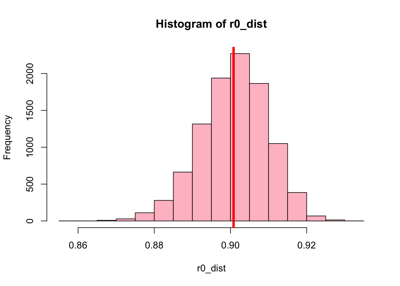
The percentile bootstrap method can be used to compute the confidence interval for the correlation coefficient:
     2.5%     97.5%
0.8820165 0.9169433
5.2.3 What you should know
Bootstrapping is a simulation-based method to investigate the distribution of a particular statistic.
The number of repetitions N controls the error of the simulation and hence the level of certainty / uncertainty in the distribution that is derived.
For very large N the distribution of the statistic is apprioximately normal
This distribution can be used to estimate a confidence interval for the statistic.
Despite many variations, all bootstrap approaches look as follows:
Obtain data sample \(x_1, x_2, \ldots,x_N\) drawn from a distribution \(F\).
Define \(u\) – the statistic computed from the sample (mean, median, etc).
Sample \(x_1^*, x_2^*, \ldots, x_n^*\) with replacement from the original data sample. Let it be \(F^*\) – the empirical (resampled) distribution.
Repeat \(N\) times (\(N\) is bootstrap iterations)
Compute \(u^*\) – the statistic calculated from each resample
Then the bootstrap principle says that:
The empirical distribution from bootstraps is approximately equal to distribution of sample data: \(F^* \approx F\).
The variation of the statistic computed from the sample \(u\) is well-approximated by the variation of the statistic computed from each resample \(u^*\). So, computed statistic \(u^*\) from bootstrapping is a good proxy for the statistic of sample data.
Sort the empirical distribution from bootstraps \(F^*\) from low to high and select those two elements from this sorted list that have 2.5% of all values below and above them, respectively (Percential bootstrapping).
5.3 Hypothesis testing through randomization
A central element of bootstrapping is randomization: the construction of new (bootstrapped) data sets by randomly selecting values from the original data set, but always with replacement sampling. A similar randomization approach, but now without replacement, can also be used to test hypothesis. To illustrate this we use a data set presented in Chowdhury et al. (2019).
Many bacteria preferentially grow within tumors and can affect tumor growth by stimulating the immune system to phagocytize tumor cells. An emerging application of synthetic biology is to genetically engineer bacteria to trigger a strong and targeted immune response within a tumor, while avoiding toxicity that occurs with the delivery of therapeutic agents via conventional means. CD47 is an anti-phagocytic receptor overexpressed in some human cancers. Studies have shown that blocking CD47 can increase phagocytosis of cancer cells, however, directly delivering CD47 blocking antibodies can result in anemia due to expression of CD47 on red blood cells. In an experiment, Chowdhury et al. (2019) genetically engineered E. coli bacteria (that colonize tumors) to release an encoded nanobody antagonist of CD47 upon lysis. The researchers conducted an in vitro study to measure the ability of this genetically engineered bacteria to increase phagocytosis rates of tumor cells. Replicated culture plates containing macrophages and A20 tumor cells were treated with one of 3 randomly assigned treatments: Phosphate-buffered saline (a control), E. coli without the nanobody antagonist of CD47, and the genetically engineered E. coli with the CD47 antagonist. The researchers measured the rate of phagocytosis of tumor cells by immune cells before and after the treatments were applied and recorded the fold change in phagocytosis.
Below is a violin plot of the results, which shows for each of the 3 treatments the distribution of relative phagocytosis rate of tumor cells by immune cells:
library(ggplot2)
data <- read.csv("data/CD47_data.csv")
# Basic violin plot
p <- ggplot(data, aes(x=Treat, y=Rel_phagocytosis, fill = Treat)) +
       geom_violin(trim = FALSE) +
        labs(x="Treatment", y = "Relative phagocytosis")
p + theme_classic() + theme(axis.text=element_text(size=16),
                            axis.title=element_text(size=18,face="bold"),
                            legend.text=element_text(size=14),
                            legend.title = element_text(size=14),
                            axis.title.y = element_text(margin = margin(t = 0, r = 10, b = 0, l = 0)),
axis.title.x = element_text(margin = margin(t = 10, r = 0, b = 0, l = 0))) 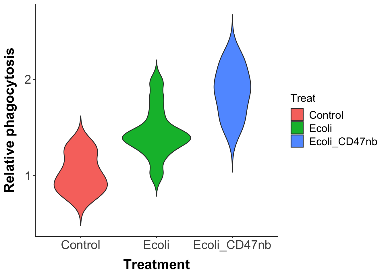
The width of the violin for a particular treatment indicates the frequency with which a particular value of the phagocytosis rate occurs.
We will here use a randomization test to test whether or not the difference between the wild-type E. coli strain and the genetically engineered E. coli strain is significant. To this end, only select the data for the two treatments with E. coli, ignoring the control treatment:
# Exclude all rows of of which the Treat label is 'Control'
Ecoli2 = data[data$Treat != 'Control',]
Ecoli2
Treat Rel_phagocytosis
12 Ecoli 1.014
13 Ecoli 1.196
14 Ecoli 1.293
15 Ecoli 1.356
16 Ecoli 1.355
17 Ecoli 1.418
18 Ecoli 1.402
19 Ecoli 1.432
20 Ecoli 1.491
21 Ecoli 1.632
22 Ecoli 1.794
23 Ecoli 1.971
24 Ecoli_CD47nb 1.456
25 Ecoli_CD47nb 1.565
26 Ecoli_CD47nb 1.590
27 Ecoli_CD47nb 1.704
28 Ecoli_CD47nb 1.817
29 Ecoli_CD47nb 1.951
30 Ecoli_CD47nb 1.951
31 Ecoli_CD47nb 1.853
32 Ecoli_CD47nb 1.979
33 Ecoli_CD47nb 2.170
34 Ecoli_CD47nb 2.161
35 Ecoli_CD47nb 2.249The data can now be analysed with a linear model applied to categorical data, as discussed in chapter 1 and 2. Using the function lm() results in:
                   Estimate Std. Error   t value     Pr(>|t|)
(Intercept)       1.4461667 0.07390557 19.567764 2.102555e-15
TreatEcoli_CD47nb 0.4243333 0.10451826  4.059897 5.211791e-04
The fitting of the linear model provides an estimate equal to 0.42433 for the treatment effect of the CD47 genetic engineering. The function lm() furthermore provided estimates for the standard error of this treatment effect and the significance level of this treatment effect. This significance test is however based on using the \(t\)-distribution, an assumption which may or may not hold for the collected data. To avoid using the assumption that the treatment effect follows the \(t\)-distribution we can use a randomization approach to test the significance of the treatment effect of CD47 genetic engineering, as illustrated in this section.
To test the significance of the treatment effect of CD47 genetic engineering, we adopt as null hypothesis \(H_0\) that CD47 genetic engineering of E. coli has no effect on the relative phagocytosis rate. If \(H_0\) holds, it implies there is no relation between the relative phagocytosis rate measured and the treatment. In other words, under \(H_0\) every value for the phagocytosis rate contained in the data set is equally likely to belong to the E. coli treatment or to the CD47 genetically engineered E. coli treatment. If the null hypothesis \(H_0\) holds, we can therefore randomly reshuffle the treatment labels of all the observations.
The following lines of code first make a copy of the original data set (cur_sample) and then samples from among the row indices without replacement. The resampled row indices are subsequently used to select the treatment labels at the corresponding rows. These resampled treatment labels are subsequently combined with the original values of the phagocytosis rate:
nsample = nrow(Ecoli2)
# Make an exact copy of the data
cur_sample = Ecoli2
# Reshuffle the labels by resampling WITHOUT replacement
cur_sample$Treat = sample(cur_sample$Treat, nsample, replace=F)
cur_sample
Treat Rel_phagocytosis
12 Ecoli_CD47nb 1.014
13 Ecoli 1.196
14 Ecoli_CD47nb 1.293
15 Ecoli_CD47nb 1.356
16 Ecoli 1.355
17 Ecoli 1.418
18 Ecoli_CD47nb 1.402
19 Ecoli 1.432
20 Ecoli 1.491
21 Ecoli_CD47nb 1.632
22 Ecoli 1.794
23 Ecoli_CD47nb 1.971
24 Ecoli_CD47nb 1.456
25 Ecoli 1.565
26 Ecoli_CD47nb 1.590
27 Ecoli 1.704
28 Ecoli_CD47nb 1.817
29 Ecoli_CD47nb 1.951
30 Ecoli 1.951
31 Ecoli 1.853
32 Ecoli_CD47nb 1.979
33 Ecoli_CD47nb 2.170
34 Ecoli 2.161
35 Ecoli 2.249Notice how as a result the labels Ecoli and Ecoli_CD47nb have been randomly reshuffled in the first column. We subsequently use the function lm() to fit a linear model to this reshuffled, randomization data set:
                     Estimate Std. Error    t value     Pr(>|t|)
(Intercept)        1.68075000 0.09751203 17.2363354 2.907787e-14
TreatEcoli_CD47nb -0.04483333 0.13790283 -0.3251081 7.481707e-01
The coefficient for the treatment effect is now quite different (-0.2913) than for the original data set. However, this value for the treatment effect is one of the possible values that can be observed if the null hypothesis \(H_0\) holds. We can now repeat this reshuffling of the treatment labels and refitting of the linear model many times (\(N=10000\) in the example code below) to build up a distribution of possible values for the treatment effect under the assumption that the null hypothesis \(H_0\) holds
nsample = nrow(Ecoli2)
N = 10000                                            # N determines number of resamplings
eff_dist = rep(NA, N)                                # Create empty vector for treatment effect
for(i in 1:N) {
  cur_sample = Ecoli2                                # Make exact copy
  cur_sample$Treat = sample(cur_sample$Treat, nsample, replace=F) # Reshuffle the labels!
  res = lm(formula = Rel_phagocytosis ~ Treat, data = cur_sample)
  eff_dist[i] = res$coefficients[2]                  # Store the treatment effect for this sample
  }
If we now plot the distribution of these randomized values for the treatment effect and compare it with the observed value for the treatment effect we have to conclude that the observed difference between E. coli and the CD47 genetically engineered E. coli is very unlikely to result from chance alone (without differences between the two types).
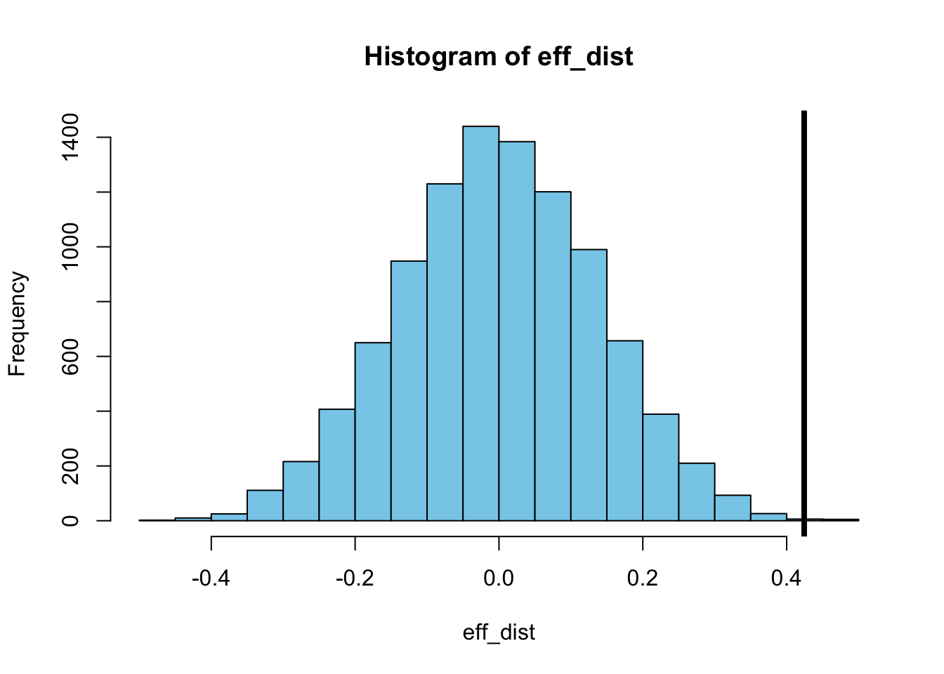
In fact, if we simply count how many of the randomized treatment effect values are smaller than the treatment effect of the original data set, we see that more than 99.9% (9993 out of 10000) of the randomized treatment effect values are smaller. In other words, the probability that the null hypothesis \(H_0\) holds is less than 0.001:
[1] 9995For such a randomization test of a particular \(H_0\) hypothesis we are not restricted to using the lm() function to compute the treatment effect size. For example, we can also compute the difference between the E. coli and the CD47 genetically engineered E. coli using the two sample test statistic provided by the function t.test(). The function call t.test(X, Y) computes for two sets of observations \(X\) and \(Y\) the value of Welch’s \(t\)-statistic, defined by the following formula:
\[ t=\dfrac{{\overline {X}}-{\overline {Y}}}{\sqrt {{s_{{\bar {X}}^{2}}+{s_{{\bar {Y}}^{2}}}}}\,} \] in which \(\overline{X}\) and \(\overline{Y}\) are the sample means of the data sets \(X\) and \(Y\) and \(s_{\bar{X}}\) and \(s_{\bar{Y}}\) are their standard errors, which are computed from the standard deviation of the sample data in the usual manner (see chapter 3.4):
\[ s_{\bar{X}} = \dfrac{s_{X}}{\sqrt{n}},\qquad s_{\bar{Y}} = \dfrac{s_{Y}}{\sqrt{n}} \] In these formula \(n\) is the length of the data sets \(X\) and \(Y\), which should be of equal length.
We can use the function t.test() to compute Welch’s \(t\)-statistic for the data on the phagocytosis rate of wild-type E. coli and CD47 genetically engineered E.coli:
res0 = t.test(Ecoli2$Rel_phagocytosis[Ecoli2$Treat == 'Ecoli'],
              Ecoli2$Rel_phagocytosis[Ecoli2$Treat == 'Ecoli_CD47nb'])
res0
    Welch Two Sample t-test

data:  Ecoli2$Rel_phagocytosis[Ecoli2$Treat == "Ecoli"] and Ecoli2$Rel_phagocytosis[Ecoli2$Treat == "Ecoli_CD47nb"]
t = -4.0599, df = 21.999, p-value = 0.0005212
alternative hypothesis: true difference in means is not equal to 0
95 percent confidence interval:
 -0.6410914 -0.2075753
sample estimates:
mean of x mean of y
 1.446167  1.870500
The value of the \(t\)-statistic equals -4.0599 and the function t.test() estimates the probability that there is no difference between the two treatments (i.e. that the \(H_0\) hypothesis holds) to equal 0.0005. However, the probability estimate depends on an assumption about the distribution of the computed \(t\)-statistic. More specifically, the assumption underlying this probability of 0.0005 is that the \(t\)-statistic follows a \(t\)-distribution with df = 21.999 degrees of freedom. We can however also use a randomization approach to estimate the probability that the observed value for the \(t\)-statistic of -4.0599 occurs under the \(H_0\) hypothesis. This randomization approach would not require the assumption that the statistic follows the \(t\)-distribution.
For the randomization approach to test the \(H_0\) hypothesis we follow exactly the same procedure as discussed above when we were using the lm() function. Randomized samples are generated from among the row indices of the original data through sampling without replacement. The resampled row indices are subsequently used to select the treatment labels at the corresponding rows and combined with the original values of the phagocytosis rate. The value of the \(t\)-statistic is subsequently calculated for this resampled data set. By repeating this procedure many times (here \(N=10000\) times) we construct a distribution of the \(t\)-statistic under the assumption that the \(H_0\) hypothesis is true.
nsample = nrow(Ecoli2)
# N determines number of resamplings
N = 10000
# Create empty vector for intercept
ttest_dist = rep(NA, N)
for(i in 1:N) {
  # Make exact copy
  cur_sample = Ecoli2
  # Reshuffle the labels by resampling WITHOUT replacement
  cur_sample$Treat = sample(cur_sample$Treat, nsample, replace=F)
  res = t.test(cur_sample$Rel_phagocytosis[cur_sample$Treat == 'Ecoli'],
               cur_sample$Rel_phagocytosis[cur_sample$Treat == 'Ecoli_CD47nb'])
  # Store the t-value of the randomized sample
  ttest_dist[i] = res$statistic
  }
Plotting this distribution together with the value of the \(t\)-statistic that was calculated for the original, unshuffled data set, shows once again that the observed difference between the wild-type E. coli and CD47 genetically engineered E.coli treatment is very unlikely to be observed under the \(H_0\) hypothesis.
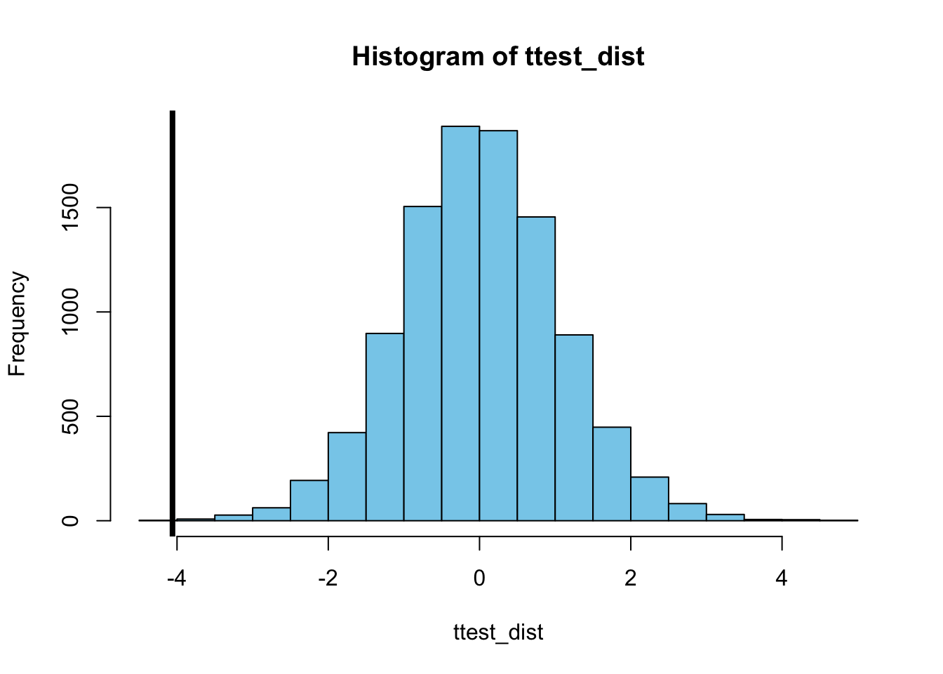
In fact, there is only a single value of the \(t\)-statistic in the distribution for the randomized data sets that is smaller than the value observed in the original data set, which suggest that the probability the \(H_0\) hypothesis holds equals 0.0001 (1 out of 10000):
[1] 05.3.1 What you should know
Randomization or permutation tests use a simulation approach to test:
whether an observed difference between two groups of observations is significant, or
whether a correlation or association between two variables is significant
Randomization or permutation tests are based on the null hypothesis \(H_0\) that there is no difference in the outcome between two groups or treatments or there is no correlation or association between two variables
Under the \(H_0\) hypothesis
measured values can be randomly reshuffled between two groups or two treatments, or
the measured value of one particular variable can be paired with any of the values of the other variable
Repeating such a randomization of the data many times builds up a distribution of the test statistic (the treatment effect when comparing two groups or the correlation coefficient between two variables) under the assumption that the \(H_0\) hypothesis holds.
Comparing the measured value of the statistic for the original data set with the distribution cnstructed using randomization provides an estimate for the likelihood for the data to occur under the \(H_0\) hypothesis
5.4 Monte Carlo process simulation
Monte Carlo simulation is a very generic name referring to any type of stochastic simulation, usually of a particular process for which the outcome is not known. Monte Carlo simulation is then used to construct a distribution of possible outcomes of the process. In statistical analysis Monte Carlo simulations are especially useful to evaluate an experimental design or to estimate parameters.
5.4.1 Evaluating an experimental design: Blood samples from elephants
The use of Monte Carlo simulation for evaluating an experimental design will be illustrated with a hypothetical example, focusing on elephants living in the Kruger National park in South Africa. Assume that there are approximately 17000 elephants living in Kruger National park (which is not so hypothetical and about right), but that 8% of these elephants are carrier of an infection with the virus Corona elephanticus (this is hypothetical for sure). To assess the variability among different strains of the virus Corona elephanticus an ecologist wants to collect blood samples of 20 infected elephants. Elephants are captured at random and a fast test is used to determine whether or not the captured elephant is infected. For simplicity we will assume that the test has an accuracy of 100% (although accounting for a smaller accuracy is not too difficult). Every captured elephant is marked, so that the same elephant is not captured again.
The question to answer is now:
How many elephants does the ecologist have to sample to collect blood from 20 infected individuals?
To simulate the sampling process that the ecologist is going to follow we define variables for the total number of elephants (Ntotal), the total number of infected elephants (NtotalInfected) and the target of infected elephants (Ntarget). At the start of the ecologist’s sampling campaign, no elephants are captured yet (Ncaptured = 0) and hence the number of infected elephants that have been captured also equals 0 (Ninfected = 0):
# Total number of elephants, the infection probability
# and the target number infected are fixed
Ntotal = 17000
NtotalInfected = 0.08 * Ntotal
Ntarget = 20

# Start with no individuals sampled or infected
Ncaptured = 0
Ninfected = 0
The sampling process carried out by the ecologist can now be simulated with a repeat loop (see the code below). The first step in this repeat loop is to randomly select a single individual from among the elephants that have not been captured yet (and are hence not marked as having been captured). This number of individuals is given by Ntotal - Ncaptured and the function sample() can be used to select a single individual from this collection. Once a single individual is selected the number of captured individuals is increased (Ncaptured = Ncaptured + 1). To determine whether the selected individual is infected or not we draw a single random number between 0 and 1 with a call to the function runif(). The fraction of infected individuals among all the individuals that have not been captured yet, equals the ratio of the number of not-captured, infected individuals and the total number of not-captured individuals ((NtotalInfected - Ninfected) / (Ntotal - Ncaptured)). If the random number generated with runif(1) is smaller than this fraction we assume that the newly captured individual is infected and hence the number of captured, infected individuals is increased (Ninfected = Ninfected + 1). The repeat loop is stopped using a break statement once the number of infected individuals captured equals the target ((Ninfected >= Ntarget)).
# Repeat the sampling until the target is reached
repeat{
  # Sample 1 individual at the time from the group
  # that has not been sampled yet
  indx = sample((1:(Ntotal - Ncaptured)), 1)
  Ncaptured = Ncaptured + 1

  # Test whether individual is infected
  # runif(1) generates 1 number between 0 and 1
  if (runif(1) < (NtotalInfected - Ninfected) / (Ntotal - Ncaptured)) {
    Ninfected = Ninfected + 1
  }

  # The break command jumps out of a loop
  if (Ninfected >= Ntarget) break
}
Ncaptured
[1] 203The above code section represents, however, a single realization of the process. In this realization only 203 elephants have to be captured to reach the target of 20 infected individuals, which is quite low. However, the sampling of individuals has a random component and this realization is therefore only one of many different realizations. In other cases we might be not so lucky and would need to capture far more elephants to reach the target of 20 infected individuals. We can now construct a distribution of possible realizations by repeating the above procedure many times a shown in the code section below (for \(N=10000\) times):
# Total number of elephants, the infection probability
# and the target number infected are fixed
Ntotal = 17000
NtotalInfected = 0.08 * Ntotal
Ntarget = 20

# N determines number of resamplings
N = 10000
# Create empty vector for results
Ncaptured_dist = rep(NA, N)
for(i in (1:N)) {

  # Start with no individuals sampled or infected
  Ncaptured  = 0
  Ninfected = 0

  # Repeat the sampling until the target is reached
  repeat{
    # Sample 1 individual at the time from the group
    # that has not been sampled yet
    indx = sample(Ntotal - Ncaptured, 1)
    Ncaptured = Ncaptured + 1

    # Test whether individual is infected
    # runif(1) generates 1 number between 0 and 1
    if (runif(1) < (NtotalInfected - Ninfected) / (Ntotal - Ncaptured)) {
      Ninfected = Ninfected + 1
    }

    # The break command jumps out of a loop
    if (Ninfected >= Ntarget) break
  }
  # Store the current result
  Ncaptured_dist[i] = Ncaptured
}
Plotting a histogram of these 10000 different realizations shows that the median value of the number of elephants that have to be captured is 246, as shown in the following plot:
hist(Ncaptured_dist, breaks = seq(60, 560, length.out = 51),
     xlim = c(60, 600), ylim = c(0, 900), col="skyblue")
abline(v=median(Ncaptured_dist), col="black",lwd=4)
text(median(Ncaptured_dist) + 5, 850, paste("Median:", median(Ncaptured_dist)),
     pos = 4, cex = 1.25)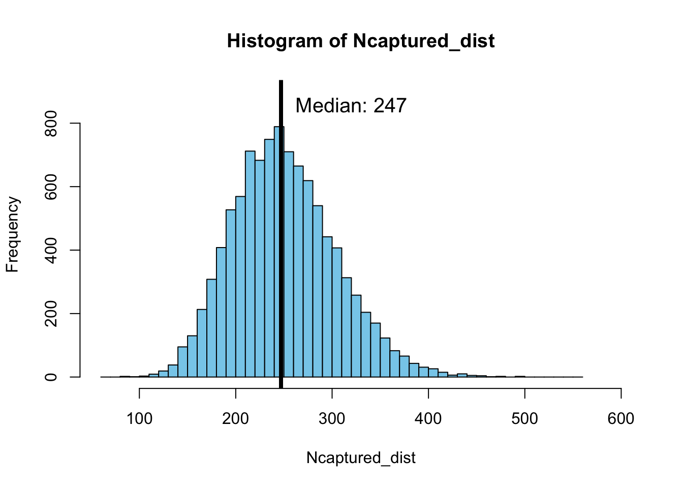
This median value is close to the expectation that we could intuitively derive by computing \(20 / 0.08 = 250\). However, the Monte Carlo simulation gives us insight into the distribution of possible outcomes and shows that sometimes we might only have to catch just over 100 elephants while in other scenarios it might take as many as 400 elephants to reach the target of 20 infected individuals. The real value of the Monte Carlo simulation approach is this insight into the distribution of possible outcomes.
5.4.2 Estimating parameters: Efficacy of the Pfizer vaccine
To illustrate the use of Monte Carlo simulation for estimation purposes, we will use the test results of a Covid-19 vaccine trial as an example. In a phase 3 trial of the Covid-19 vaccine produced by Pfizer, a randomized, double-blind test was carried out, in which individuals that signed up for the test were randomly given an injection with the vaccine or with a placebo. Neither the individuals receiving an injection nor the doctors administering them knew whether they had received a vaccine or not (hence the adjective ``double-blind’’). A total of 43210 individuals received an injection in this phase 3 trial. The company Pfizer had determined that the trial would be stopped and evaluated when a total number of 170 participants in the trial had become infected with Covid-19 and hence tested positive. Participants in the trial were continuously monitored for Covid-19 infection.
After the completion of the trial, when 170 individuals had become infected with Covid-19, it turned out that 21380 individuals had received the vaccine (\(N_v = 21380\)), while 21830 individuals had received a placebo (\(N_p = 21830\)). Of the 170 individuals infected with Covid-19, 162 individuals belonged to the group that had received a placebo, while 8 individuals belonged to the group that had received the vaccine.
The question to answer with Monte Carlo simulation is:
What is the most likely value and the confidence interval of the probability that an individual that received the vaccine becomes infected with Covid-19, relative to the infection probability of individuals that did not receive the vaccine?
To start answering this question we set the infection probability of individuals that received a placebo equal to 1, while the infection probability of individuals that received a vaccine is set equal to some value, say \(p = 0.04\). This probability that a vaccinated individual gets infected is therefore relative to the infection probability of an unvaccinated individual. Moreover, the value of \(p = 0.04\) is just an arbitrary choice, later the computations will be repeated for a range of different \(p\) values.
The code shown below computes a single simulated realization of the infection process that could have occurred within this trial for a relative infection probability of vaccinated individuals equal to \(p = 0.04\). Check the code line by line while reading the explanation that follows.
In the code the variables Nplacebo and Nvaccine are set to the number of individuals that received a placebo and a vaccine, respectively, while the variable Pinfect is set to the relative infection probability of vaccinated people \(p = 0.04\) and the variable Ntarget is set to the target value of 170 infected individuals which Pfizer had decided as the threshold value at which the trial would be stopped. The infection process is now simulated using a repeat loop that is stopped by means of a break statement if the total number of infected individuals equals this target value of 170. The infection process starts out without any infected individuals among the individuals that received a placebo (NinfectP = 0) and among the vaccinated people (NinfectV = 0).
Within the repeat loop as a first step the number of individuals is computed in the placebo and the vaccinated group that have not been infected yet by subtracting from the total number of individuals in these two groups the number of infected individuals in the two groups (NnotillP = Nplacebo - NinfectP and NnotillV = Nvaccine - NinfectV). The sum of these values gives the total number of individuals that is not infected yet (Nnotill = NnotillP + NnotillV). The function sample() is used to select the index of a single individual from this group of still uninfected individuals. If this randomly selected index is in the range between 1 and the value of the variable NnotillP the selected individual has received a placebo, if the index is larger than the value of the variable NnotillP the selected individual has received a vaccine. (As an aside: This choice of the implementation is arbitrary: for the same token we could have assumed that if the index of the randomly selected index is in the range between 1 and the value of the variable NnotillV the selected individual has received a vaccine, while if the index is larger than the value of the variable NnotillV the selected individual has received a placebo). If an individual is selected that has received a placebo it gets infected with probability 1 and the variable NplaceboP is increased by 1. For an individual that received a vaccine, the probability to get infected is smaller than 1 and hence we generate a random value between 0 and 1 using the function call runif(1). Only if the result of this call is smaller than the infection probability Pinfect (\(p = 0.04\)) the vaccinated individual gets infected and the number of infected individuals that received a vaccine (NinfectedV) is increased by 1. This random sampling of individuals is continued until the total number of individuals that has become infected NinfectP + NinfectV reaches the target value of 170 individuals.
# Assume the total number of individuals receiving a placebo and a vaccine is fixed
Nplacebo = 21830
Nvaccine = 21380
Ntarget  = 170
NVobs    = 8

Pinfect  = 0.04

# Start with no individuals infected
NinfectP = 0
NinfectV = 0

# Repeat the sampling until the target is reached
repeat{

  # Sample 1 individual at the time from the group that has not fallen ill yet
  NnotillP = Nplacebo - NinfectP
  NnotillV = Nvaccine - NinfectV
  Nnotill  = NnotillP + NnotillV
  indx = sample((1:Nnotill), 1)

  # Test whether an individual received a placebo
  if (indx <= NnotillP) {
    NinfectP = NinfectP + 1
  } else {
    # Test whether individual that received vaccine gets infected
    if (runif(1) < Pinfect) {
      NinfectV = NinfectV + 1
    }
  }

  # The break command jumps out of a loop
  if ((NinfectP + NinfectV) >= Ntarget) break
}[1] 163 7The above code section represents, however, a single realization of the infection process, resulting in 163 individuals getting infected that received a placebo and 7 individuals that received a vaccine. As in the previous subsection we can construct a distribution of the possible realizations by repeating the above procedure many times as shown in the code section below (for \(N=5000\) times). To store the results a matrix is constructed with two columns of empty values, in which the first column will hold the number of infected individuals that received a placebo and the second column the number of individuals that received a vaccine.
# Assume the total number of individuals receiving a placebo and a vaccine is fixed
Nplacebo = 21830
Nvaccine = 21380
Ntarget  = 170
NVobs    = 8

Pinfect  = 0.04

# N determines number of resamplings
N = 5000
# Create empty vector for results
Ninfect_dist = matrix(NA, nrow = N, ncol = 2)

for(i in (1:N)) {

  # Start with no individuals infected
  NinfectP = 0
  NinfectV = 0

  # Repeat the sampling until the target is reached
  repeat{

    # Sample 1 individual at the time from the group that has not fallen ill yet
    NnotillP = Nplacebo - NinfectP
    NnotillV = Nvaccine - NinfectV
    Nnotill  = NnotillP + NnotillV
    indx = sample((1:Nnotill), 1)

    # Test whether an individual received a placebo
    if (indx <= NnotillP) {
      NinfectP = NinfectP + 1
    } else {
      # Test whether individual that received vaccine gets infected
      if (runif(1) < Pinfect) {
        NinfectV = NinfectV + 1
      }
    }

    # The break command jumps out of a loop
    if ((NinfectP + NinfectV) >= Ntarget) break
  }

  # Store the current result
  Ninfect_dist[i,] = c(NinfectP, NinfectV)
}
colnames(Ninfect_dist) <- c("Placebo", "Vaccine")
To inspect the result we plot a histogram of the number of vaccinated individuals among the total group of 170 individuals that got infected observed in all these 5000 different realizations:
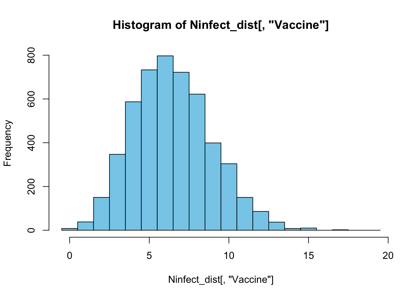
The histogram shows that for \(p = 0.04\) most often only 6 vaccinated individuals would be among the total group of 170 infected individuals. To obtain an estimate for the relative probability of vaccinated individuals to get infected we can now repeat the procedure above for a range of different infection probability values \(p=0, 0.001, 0.002, \ldots, 0.099, 0.1\) and check for each value of \(p\) which fraction of the realizations resulted in 8 vaccinated individuals to become infected, as was observed in the real trial. By defining the variable NVobs equal to 8, the fraction of realizations that resulted in 8 vaccinated individuals to become infected can be calculated with the statement:
[1] 0.1244The resulting value for this fraction is stored in the second column of a matrix Pinfect, the first column of which contains the value of the corresponding infection probability \(p\). The following code carries out the computations for the range of infection probabilities \(p=0, 0.001, 0.002, \ldots, 0.099, 0.1\) (this code section takes a very long time to complete, because it contains a repeat loop within a for loop that is in turn contained within another for loop. Be aware of that when trying to run the code yourself).
# Assume the total number of individuals receiving a placebo and a vaccine is fixed
Nplacebo = 21830
Nvaccine = 21380
Ntarget  = 170
NVobs    = 8

Plow = 0.0
Phigh = 0.1
Pnr = 101
Pinfect = matrix(NA, nrow = 101, ncol = 2)
Pinfect[,1] = seq(Plow, Phigh, length.out = Pnr)

# N determines number of resamplings
N = 5000
# Create empty vector for results
Ninfect_dist = matrix(NA, nrow = N, ncol = 2)

for (p in (1:Pnr)) {

  for(i in 1:N){

    # Start with no individuals infected
    NinfectP = 0
    NinfectV = 0

    # Repeat the sampling until the target is reached
    repeat{

      # Sample 1 individual at the time from the group that has not fallen ill yet
      NnotillP = Nplacebo - NinfectP
      NnotillV = Nvaccine - NinfectV
      Nnotill  = NnotillP + NnotillV
      indx = sample((1:Nnotill), 1)

      # Test whether an individual received a placebo
      if (indx <= NnotillP) {
        NinfectP = NinfectP + 1
      } else {
        # Test whether individual that received vaccine gets infected
        if (runif(1) < Pinfect[p , 1]) {
          NinfectV = NinfectV + 1
        }
      }

      # The break command jumps out of a loop
      if ((NinfectP + NinfectV) >= Ntarget) break
    }

    # Store the current result
    Ninfect_dist[i,] = c(NinfectP, NinfectV)
  }
  colnames(Ninfect_dist) <- c("Placebo", "Vaccine")

  # Store the current result
  Pinfect[p ,2] = sum(Ninfect_dist[, "Vaccine"] == NVobs) / N
}
The last step in the estimation process is to plot for each value of the infection probability \(p\) the fraction of realizations that resulted in exactly 8 vaccinated individuals to get infected:
par(mar = c(6,6,1,1))
plot(Pinfect, pch = 19, xlab ="Infection probability", ylab = "Likelihood", cex.lab = 1.6, yaxt = "n", cex.axis = 1.25)
axis(2, las = 2, cex.axis = 1.25)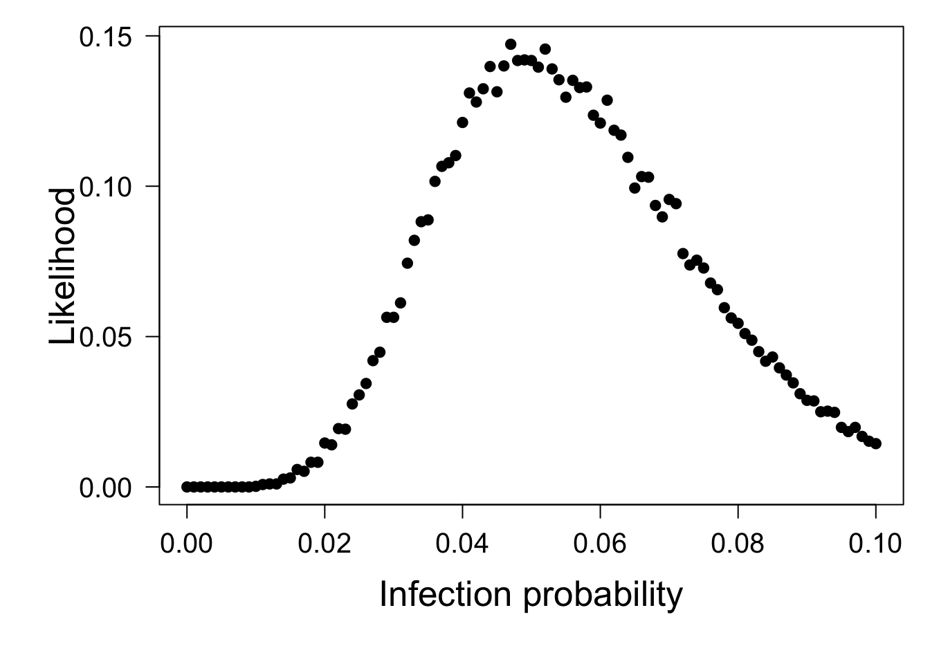
This plot show for each value of the relative infection probability the likelihood of the outcome of 8 vaccinated individuals and 162 individuals from the placebo group to become infected, as was observed in the real trial. The maximum of the likelihood curve occurs at \(p=0.047\):
[1] 0.047However, if we inspect the entire plot we also observe that the likelihood value varies quite a bit from one value of the infection probability \(p\) to the other, such that there is no clear single value with the highest likelihood. The relative infection probability of vaccinated individuals is therefore around 0.05 compared to unvaccinated individuals, but the simulation results are not sufficiently accurate to provide a more precise estimate of this probability. We can however estimate a confidence interval by checking for which values of the probability the likelihood of the outcome of 8 vaccinated individuals and 162 individuals from the placebo group to become infected is larger than or equal to 0.025.
[1] 0.024 0.0935.4.3 What you should know
Monte Carlo simulations can be used to simulate any process, of which the outcome is influenced by some source of stochasticity
Repeating the simulation of the process many times, generates a distribution of possible outcomes
This distribution can in turn be used to analyze, for example, an experimental design or to estimate parameters, as illustrated by the two examples in this section
The application of Monte Carlo simulations is however not limited to evaluating experimental designs or estiamting parameters, the applicabilition of Monte Carlo simulation method is only limited by our own imagination