2.5.3. Cumulative Distribution Function

The cumulative distribution function brings the discrete and continuous RV’s together. For a RV \(X\) the cumulative distribution function (often called the distribution function) is defined as:

\[F_X(x) = \P(X\leq x)\]

Note that \(x\in\setR\) even in case \(X\) is a discrete RV. We have:

\[\begin{split}F_X(x) = \begin{cases} \sum_{k=-\infty}^{\lfloor x\rfloor} p_X(k) &\text{Discrete $X$}\\ \int_{-\infty}^{x} f_X(y)\, dy &\text{Continuous $X$} \end{cases}\end{split}\]

Below a probability mass function \(p_X\) is plotted and the corresponding \(F_X\).

Show code for figure

import numpy as np
import matplotlib.pyplot as plt

plt.clf()

pX = np.array([0,0,0,0,1,2,4,5,7,6,5,3,1,0,0,0])
pX = pX / np.sum(pX)
x = np.arange(len(pX))-7
cpX = np.cumsum(pX)

plt.subplot(211)
plt.title(r"Probability Mass Function")
plt.stem(x, pX, use_line_collection=True)
plt.subplot(212)
plt.title(r"Cumulative Distribution Function")
plt.step(x, cpX, where='post')
plt.savefig('source/figures/cumprobfunc.png')

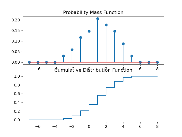
Fig. 2.5.3 Cumulative Probability Function.

And a plot of a probability density function and its corresponding cumulative distribution function.

Show code for figure

import numpy as np
import matplotlib.pyplot as plt
#
# I am cheating by calculating things for a sampled function...
# ONLY LOOK AT THE PLOTS...
#

x = np.linspace(-8, 8, 1000)
pX = np.piecewise(x, [x<-4, np.logical_and(x>=-4, x<4), x>=4],
                  [0, lambda x: 16-x**2, 0])
pX = pX / np.sum(pX)
cpX = np.cumsum(pX)

plt.clf()
plt.subplot(211)
plt.title(r"Probability Density Function")
plt.plot(x,pX)
plt.subplot(212)
plt.title(r"Cumulative Distribution Function")
plt.step(x, cpX, where='post')
plt.savefig('source/figures/continuous_cdf.png')

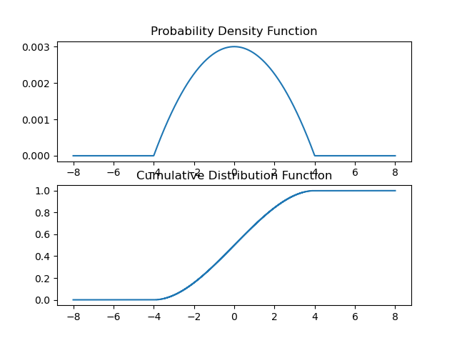
Fig. 2.5.4 Cumulative Probability Function.

The cumulative distribution function follows from the probability density function by integration. We can go the other way as well:

\[f_X = \frac{d}{dx} F_X\]

With some mathematical leniency we can say that this also holds for a discrete random variable. [1]

Footnotes

[1]

Representing a discrete random variable as a continous random variable can be done using dirac delta pulses. The dirac delta function \(\delta\) is defined with the integral property:

\[\int_{-\infty}^{\infty} f(x) \delta(x) dx = f(0)\]

The dirac delta function is zero everywhere except at the origin. The value in the origin is ill defined but the integral over an infinitesimally small interval from \(-\epsilon\) to \(+\epsilon\) of \(\delta(x)\) equals one. For some intuitive understanding of the dirac delta function consider the Gaussian function in the limit for \(\sigma\rightarrow0\).

With the use of the dirac delta function we can define the derivative of the cumulative distribution of a discrete random variable with probability mass function \(p_X(x)\) and cumulative distribution \(F_X(x)\) as

\[\frac{d F_X(x)}{dx} = \sum_{k=-\infty}^{\infty} p_X(k) \delta(x-k)\]

Note that for the right hand side is a representation of the discrete probability mass function \(p_X(k)\) as a continuous probability density function.