2.5.1. Discrete Random Variables

A discrete random variable \(X\) maps the elementary events \(u\in U\) unto a value in \(\setZ\). i.e. \(X: u\in U \mapsto X(u)\in\setZ\). Note that the random variable \(X\) in iteself is not an event. We can specify an event \(A\), associated with outcome \(X=x\), by specifying

\[A = \{ u \bigm| X(u)=x \}\]

We will most often abbreviate this and write the event \(A\) as \(X=x\). Carefully note the distinction between capital \(X\) and \(x\). The capital \(X\) always refers to random variables and lower case letters refer to values from the range of the mapping \(X\).

A discrete variable is completely characterized in case for all \(x\in\setZ\) we specify \(\P(X=x)\). We will do this with the probability mass functions \(p_X\):

\[p_X(x) = \P(X=x)\]

As an example consider our fair die again, there we have:

\[\begin{split}p_X(x) = \begin{cases} 0 &: x < 1\\ \frac{1}{6} &: 1\leq x \leq 6\\ 0 &: x > 6 \end{cases}\end{split}\]

Show code for figure

import numpy as np
import matplotlib.pyplot as plt

plt.clf()

x = np.arange(-5, 12)
p = np.zeros_like(x, dtype=float)
p[np.logical_and(x>=1, x<=6)] = 1/6
plt.stem(x,p)
plt.savefig('source/figures/pmsdice.png')

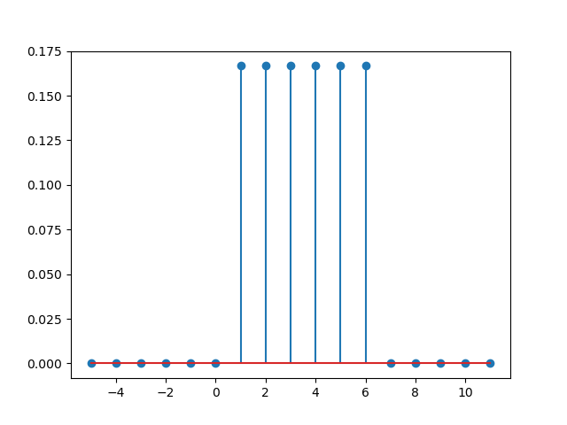
Fig. 2.5.1 Probability Mass Function corresponding with the discrete random variable that denotes the value thrown with a die.

Note that we assume that the events \(X=x_1\) and \(X=x_2\) are disjunct in case \(x_1\not=x_2\) and futhermore that all \(X=x\) for \(x\in\setZ\) form a partition of \(U\) and therefore:

\[\sum_{x\in\setZ} p_X(x) = 1\]

As an example of a discrete random variable let us set a simple random experiment. We throw with two dice and count the number of both die.

\[X=x\quad\text{$x$ is the sum of both dice}\]

It is evident that \(p_X(x)=0\) for \(x<2\) and \(x>12\). Later on in this chapter we will discuss how to calculate the probabilities for \(2\le x\le 12\). Here we will assume that we are able to simulate this random experiment by randomly generating two numbers in the range from 1 to 6 and adding these numbers. With this simulation we can estimate the probabilities based on our frequentist view on probability. The result is shown in the figure below.

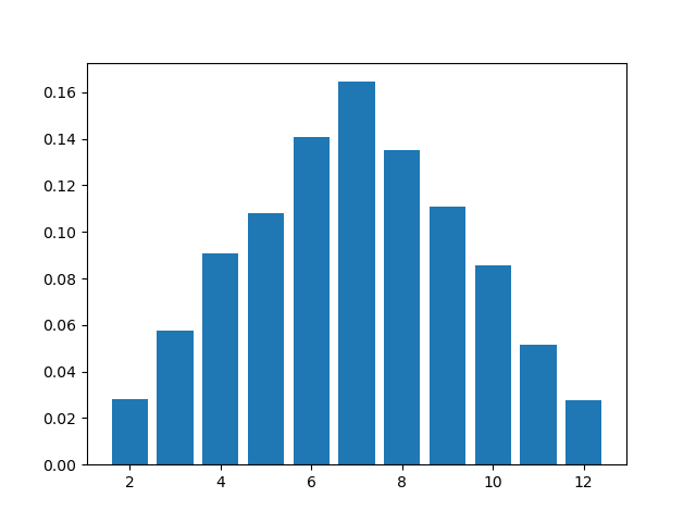
Fig. 2.5.2 Estimated Probability Mass Function \(p_X(x)\) where \(X\) is the sum of two dice.

Carefully note that this is only an estimate of the probability mass function. In this case it is easy to calculate the exact function (we will do that in a later section) in other situations observing a random experiment and estimating the probability mass function from the sample is needed.