2.11.1. Expectation and (Co)variance

2.11.1.1. The Expectation of Random Vectors

Consider two vector values \(\v x_1\) and \(\v x_2\). The average or mean of these vectors is defined as the vectorial mean: i.e. first add the two vectors elementwise and then divide all elements by two. In vectorial notation:

\[\bar{\v x} = \tfrac{1}{2}(\v x_1+\v x_2)\]

The mean of two vectors is the vector that ends precisely inbetween the two vectors. If we take the mean of several random vectors:

\[\bar{\v x} = \tfrac{1}{n}(\v x_1+\cdots+\v x_n)\]

the mean will be ‘in the center’ of the cluster of points (vectors).

In case we take the mean of an infinite number of values and all the values are independent and identically distributed the mean will converge to the expectation of the random vector. For a discrete random vector we have:

\[\E(\v X) = \sum_{\v x} \v x\, p_{\v X}(\v x)\]

For a continuous random vector the summation changes to an integration:

\[\E(\v X) = \int_{\setR^n} \v x\, f_{\v X}(\v x) d\v x\]

Note that the above integral is a short hand notation for \(n\) integrals:

\[\begin{split}\E(\v X) = \int_{\setR^n} \v x \, f_{\v X}(\v x) d\v x = \matvec{c}{ \int_{\setR^n} x_1\, f_{\v X}(\v x) d\v x \\ \int_{\setR^n} x_2\, f_{\v X}(\v x) d\v x \\ \vdots \\ \int_{\setR^n} x_n\, f_{\v X}(\v x) d\v x }\end{split}\]

We thus see that the expectation of a vector random variable is the vector of the expectations of the vector elements (each a random variable):

\[\begin{split}\E(\v X) \equiv \E( \matvec{c}{X_1\\ \vdots \\ X_n} ) = \matvec{c}{\E(X_1)\\ \vdots \\ \E(X_n)}\end{split}\]

We have seen before that the expectation of a weighted sum of random variables equals the weighted sum of the expectations:

\[\E( \sum_{i=1}^{n} a_i \, X_i ) = \sum_{i=1}^{n} a_i \,\E( X_i )\]

This results generalises to the following result for the expectation of a random vector:

\[\E( A\v X) = A \E(\v X)\]

where \(A\) is any \(m\times n\) real matrix and \(n\) is the dimension of vector \(\v X\).

2.11.1.2. The (Co)Variance of Random Vectors

The notion of variance is not so easy to deal with for random vectors. Consider the scatter plots of the samples of two different 2D random vectors in the figure below.

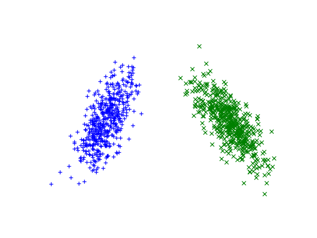
For a scalar random variable the variance is defined with \(\Var(X) = E((X-E(X))^2)\) and captures the mean (quadratic) deviation of the samples from the expected value. For a random vector the deviation from the mean is the vector \(\v X - E(\v X)\) and thus we cannot take the square of it. We could define something like the expectation of the square of the norm of this vector:

\[E( \|\v X-E(\v X)\|^2 )\]

to indicate the spread around the expected value. This measure however cannot make a distinction between the two distributions in the above figure.

So one number does not suffice to capture the variance of random vectors. Not even the variances of all random variables in the vector can complete capture this. What we miss is the correlation of the individual elements in the random vector.

We start with two random variables \(X_1\) and \(X_2\). Now consider the variance of \(X_1+X_2\):

\[\begin{split}\Var(X_1+X_2) &= E( (X_1+X_2-E(X_1+X_2))^2 ) \\ &= E( ( X_1-E(X_1) + X_2-E(X_2) )^2 ) \\ &= E( (X_1-E(X_1))^2 + (X_2-E(X_2))^2 + 2(X_1-E(X_1))(X_2-E(X_2)) ) \\ &= E( (X_1-E(X_1))^2 ) + E( (X_2-E(X_2))^2 ) + 2 E((X_1-E(X_1))(X_2-E(X_2))) \\ &= \Var(X_1)+\Var(X_2) + 2 E((X_1-E(X_1))(X_2-E(X_2)))\end{split}\]

The last expectation term is called the covariance of the random variables \(X_1\) and \(X_2\).

\[\Cov(X_1,X_2) = E((X_1-E(X_1))(X_2-E(X_2)))\]

The covariance is (and i quote from Wikipedia) “a measure of how much two random variables change together. If the greater of one variable mainly correspond with the greater values of the other variable, and the same holds for the smaller values, i.e., the variables tend to show similar behavior, the covariance is positive. In the opposite case, when the greater values of one variable mainly correspond to the smaller values of the other, i.e., the variables tend to show opposite behavior, the covariance is negative. The sign of the covariance therefore shows the tendency in the linear relationship between the variables. The magnitude of the covariance is not easy to interpret.”

Two random variables whose covariance is zero are called uncorrelated. It should be noted that independence and correlation are related concepts but are not the same. Any two random variables that are independent are uncorrelated but the reverse is not nescessarily true (see the Wikipedia entry on Correlation and Dependence).

Now consider a random vector \(\v X\). Here we can distinguish the variances \(\Var(X_i)\) (for \(i=1,\dots,n\)) and covariances \(\Cov(X_i,X_j)\). All these (co)variances are gathered in the covariance matrix:

\[\begin{split}\Cov(\v X) = \matvec{cccc}{ \Cov(X_1,X_1) & \Cov(X_1,X_2) & \cdots & \Cov(X_1,X_n) \\ \Cov(X_2,X_1) & \Cov(X_2,X_2) & \cdots & \Cov(X_2,X_n) \\ \vdots & \vdots & \ddots & \vdots \\ \Cov(X_n,X_1) & \Cov(X_n,X_2) & \cdots & \Cov(X_n,X_n)}\end{split}\]

Because \(\Cov(X,X)=\Var(X)\), the diagonal elements of the covariance matrix are the variances of the scalar random variables in the random vector \(\v X\).

In matrix-vector notation the covariance matrix can be written as:

\[\Cov(\v X) = E((\v X-E(\v X))(\v X-E(\v X))\T)\]

It is (again) easy to prove that in case random vector \(\v X\) has covariance matrix \(\Cov(\v X)\) we have that:

\[\Cov(A\v X) = A\Cov(\v X) A\T\]

If you keep in mind that \(\Cov(aX)=a^2 \Cov(X)\) for a scalar random variable the fact that the covariance matrix for \(A\v X\) contains the elements of \(A\) in a quadratic manner might seem reasonable.

As promised the proof is simple:

\[\begin{split}\Cov(A\v X) &= E( (A\v X-E(A\v X))(A\v X-E(A\v X))\T ) \\ &= E( (A\v X-A E(\v X))(A\v X-A E(\v X))\T ) \\ &= E( A(\v X- E(\v X))(\v X- E(\v X))\T A\T ) \\ &= A E( (\v X- E(\v X))(\v X- E(\v X))\T )A\T \\ &= A \Cov(\v X) A\T\end{split}\]

2.11.1.3. Directional variance

Consider a random vector \(\v X\) with a distribution with expectation and covariance matrix given by

\[\begin{split}\mu &= \matvec{c}{8\\5}\\ \Sigma &= \matvec{cc}{1 & 1 \\ 1 & 2}\end{split}\]

In the scatter plot of 500 samples from this distribution we observe that the variance is not equal for all directions in the plane. In the diagonal direction (from bottom left to top right) there is a large spread (variance) whereas in the other diagonal direction the variance is smaller.

In this section we will quantify this observation. Consider a random vector \(X\) with expectation \(\v \mu = E(\v X)\) and covariance matrix \(\v\Sigma = \Cov(\v X)\).

To quantify the variance in direction \(\v r\) (where \(\|\v r\|=1\)) we look at the random variable \(Y=\v r\T \v X\), i.e. we project the random vector on the line through the origin in the \(\v r\) direction.

It is simple to prove that

\[\begin{split}\Var(Y) &= \Var(\v r\T \v X) \\ &= \Cov(\v r\T \v X) \\ &= \v r\T \Cov(\v X) \v r\end{split}\]

based on the observation that for a scalar random variable the variance equals the covariance ‘matrix’ and by using the property that \(\Cov(A\v X) = A \Cov(\v X) A\T\)

This results shows that the covariance matrix is all we need to calculate the scalar variance of a multivariate dataset projected on any direction.

2.11.1.4. Correlation and Dependency

Two random variables \(X_i\) and \(X_j\) (for \(i\not= j\)) in the random vector \(\v X\) are said to be uncorrelated in case \(\Cov(X_i,X_j)=0\). In case the covariance matrix is a diagonal matrix all elements in the random vector are uncorrelated.

The fact that two random variables are uncorrelated does not imply that these variables are independent. On the other hand we do have that independence implies that the random variables are uncorrelated. First we rewrite the definition of the covariance:

\[\begin{split}\Cov(X,Y) &= E( (X-E(X))(Y-E(Y)) ) \\ &= E( XY - XE(Y) - YE(X) + E(X)E(Y) ) \\ &= E(XY) - E(X)E(Y) - E(X)E(Y) + E(X)E(Y) \\ &= E(XY) - E(X)E(Y)\end{split}\]

In case \(X\) and \(Y\) are independent we have:

\[E(XY) = \int_\setR \int_\setR x\,y\,f_{XY}(x,y) dx dy\]

Independence of both random variables means that the joint probability density can be written as the product of the marginal densities:

\[\begin{split}E(XY) &= \int_\setR \int_\setR x\,y\,f_{XY}(x,y) dx dy \\ &= \int_\setR \int_\setR x\,y\,f_{X}(x)f_{Y}(y) dx dy \\ &= \int_\setR x\,f_{X}(x)dx \int_\setR y\,)f_{Y}(y) dy \\ &= E(X)E(Y)\end{split}\]

Substituting this in the expression for the covariance that we have derived just above we get that \(\Cov(X,Y)=0\) for independent random variables.

As a simple example to illustrate that uncorrelated random variables can be dependent consider \(X\sim\Normal(0,\sigma^2)\) and \(Y=X^2\). By construction there are clearly not independent! We can calcatute the covariance as:

\[\begin{split}\Cov(X,Y) &= E(XY)-E(X)E(Y) \\ &= E(X^3) - 0 \\ &= \int_{-\infty}^{\infty} x^3 f_{X}(x) dx \\ &= \frac{1}{\sigma\sqrt{2\pi}}\int_{-\infty}^{\infty} x^3 e^{-\frac{x^2}{2\sigma^2}}dx\\\end{split}\]

We don’t have to calculate this integral explicitely. Observe that the integrand is an asymmetrical function and thus contributions to the integral for positive and negative x-values cancel and thus the integral equals zero:

\[\Cov(X,Y)=0\]

We thus have dependent random variables that are uncorrelated.

2.11.1.5. Estimation of \(E(\v X)\) and \(\Cov(\v X)\)

Let \(\v X\) be a vectorial random variable with expectation \(E(\v X)\) and covariance matrix \(\Cov(\v X)\). Given the pmf or pdf of \(\v X\) both expectation and covariance can be calculated. In practice however, we often do not know the pdf or pmf but instead we have to approximate these as function of a sample of \(\v X\).

Given a sample of \(\v X\) with \(m\) vectors:

\[\v x\ls 1, \ldots, \v x\ls m\]

the expectation can be estimated as the mean \(\bar{\v x}\):

\[\widehat{E(\v X)} = \bar{\v x} = \frac{1}{m} \sum_{i=1}^{m} \v x\ls i\]

and the covariance matrix as:

\[\widehat{\Cov(\v X)} = S = \frac{1}{m} \sum_{i=1}^{m} (\v x\ls i - \bar{\v x})(\v x\ls i - \bar{\v x})\T\]