2.11.2. Normal Distributed Random Vectors

2.11.2.1. Definition

The multivariate normal distribution of an n-dimensional random vector is defined as:

\[f_{\v X}(\v x) = \frac{1}{(2\pi)^{n/2} |\v \Sigma|^{1/2}} \exp\left( -\tfrac{1}{2}(\v x - \v \mu)\T \v \Sigma^{-1} (\v x-\v\mu) \right)\]

We can also define the multivariate normal distribution with the statement that a random vector \(\v X\) has a normal distribution in case every linear combination of its components is normally distributed, i.e. for any scalar vector \(a\) the univariate (or scalar) random variable \(Y = \v a\T\v X\) is normally distributed.

The normal distribution is completely characterized with its expectation and (co)variance:

\[\begin{split}\E(\v X) = \v\mu \\ \Cov(\v X) = \v\Sigma\end{split}\]

As an example consider the two dimensional normal distribution with

\[\begin{split}\v \mu = \matvec{c}{8\\5}\\ \Sigma = \matvec{cc}{1 & 1 \\ 1 & 2}\end{split}\]

Plotting 500 samples from this distribution gives an impression of the probability density function. Where a lot of samples cluster on the plane the density will be high and it will be lower where less samples are.

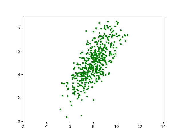
From the scatter plot we can infer that the mean value of the samples is indeed somewhere near the point \((8,5)\). The distribution is clearly elongated in an (almost) diagonal direction. In the next section we will show how to relate the covariance matrix with the ‘shape’ of the scatterplot.

For this distribution we can make a plot of the probability density function itself where we now assume that \(\v\mu=\v 0\):

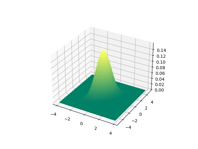
If you run this code and plot the probability density function in a separate window (or using %matplotlib notebook) you can interactively scale and rotate the plot to make the 3D geometry better visible.

2.11.2.2. Geometry

In order to get a feeling for the ‘shape’ of the distribution we look at the isolines of the probability density function \(f_{\v X}(\v x)=\text{constant}\). Assume that \(\v \mu = \v 0\), i.e. the distribution is centered at the origin. Then

\[\v x\T \Sigma\inv \v x = \text{constant}\]

Since the covariance matrix is symmetric (and thus its inverse is too) we recognize a quadratic form: \(\v x\T Q \v x\) with a symmetric matrix \(Q=\Sigma\inv\).

As an example consider the two dimensional case with zero mean and diagonal covariance matrix

\[\begin{split}\Sigma = \begin{pmatrix}4&0\\0&9\end{pmatrix}\end{split}\]

The probability density function then has curves of constant value defined by:

\[\left(\frac{x_1}{2}\right)^2 + \left(\frac{x_2}{3}\right)^2 = \text{constant}\]

Which is an axis aligned ellips that is more elongated in the \(x_2\) direction. In 3D space we get an ellipsoid surface and in nD we talk of hypersurfaces of constant probability density.

In the figure below some ellipses of constant probability density are shown for the same 2D pdf as used in the previous section.

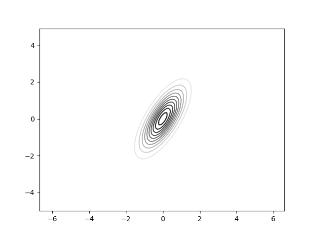
Remember from linear algebra class that a quadratic form can always be diagonalized, i.e. we can find an orthogonal basis in which the covariance matrix is diagonal. Thus the non diagonal elements in the covariance matrix determine the rotation of the ellipsoid shape of the (hyper) surfaces of constant probability density.

For any symmetric real valued matrix, as the covariance matrix is, we can write:

\[\Sigma = U\; D\; U\T\]

where \(U\) is the matrix whose columns are the eigenvectors of \(\Sigma\) and \(D\) is a diagonal matrix whose elements are the eigenvalues of \(\Sigma\):

\[\begin{split}U &= \begin{pmatrix}\v u_1 & \cdots & \v u_n\end{pmatrix}\\ D &= \begin{pmatrix}\lambda_1 & &\\&\ddots&\\&&\lambda_n\end{pmatrix}\end{split}\]

where \(\v u_i\) is the i-th eigenvector with eigenvalue \(\lambda_i\).

So in case \(\v X\) is normally distributed with zero mean \(\v\mu=\v 0\) and covariance matrix \(\Sigma\) then \(\v Y = U\T \v X\) has covariance matrix:

\[\Cov(\v Y) = \Cov(U\T \v X) = U\T \Sigma U = D\]