7. Histogram of Oriented Gradients¶

In this exercise you are asked to implement the calculation of an Histogram of Oriented Gradients. In the web article Histogram of Oriented Gradients an implementation is discussed that also explains the concepts quite clearly.

The aforementioned web article is using functions from OpenCV. In this exercise you are not allowed to use OpenCV functions.

First read the web article and then continue with the steps below that follow the steps in the web article.

7.1. Step 1: Preprocessing¶

I couldn’t find the bolt.png image that is used but i found the bolt2.png image.

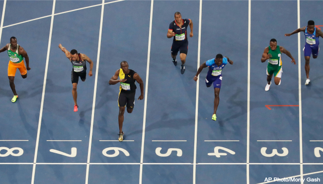
Crop the outline of one of the runners as is done in the webarticle (i.e. in a 1:2 aspect ratio!) and warp (resize) it to a size of 64x128 pixels (colums x rows). Like in the article you should select a rather large border around the running figure.

7.2. Step 2: Calculate the Gradient Images¶

We can do better than just using simple central difference schemes as used in the web article. Calculate the gradient using Gaussian derivatives (at a small scale).

There is one snag in this. The OpenCV code deals with color images in a rather peculiar way. It calculates the derivatives for each color channel separately. Combination of the color channels to come up with one gradient magnitude and one gradient angle is not defined clearly (imho).

We make a shortcut here. We first reduce the color image to a gray value image. And use this scalar image from here on.

Visualize the gradient components \(f_x\) and \(f_y\) and the gradient magnitude.

Write a simple function mag, angle = cart2polar(fx, fy). In the web article the angle is in degrees. I strongly suggest you do all your programming with angles in radians. Make sure that the angle that is returned is an orientation angle in the range from \(0\) to \(\pi\).

7.3. Step 3: Calculate HOG in 8x8 Cells¶

Write a function HOG8x8(gx, gy) that takes two a scalar 8x8 images as input where gx is the derivative in x direction and gy the derivative in y direction. The function should return a 9 bin histogram (as a vector of shape (9,)) as explained in the web article.

Note that the histogram function from numpy has a keyword argument weights and that is just what is needed in this application!

Test your function before moving on:

gx = ones((8,8))*cos(pi/4)
gy = ones((8,8))*sin(pi/4)
h = HOG8x8(gx, gy)

What would you expect to be the result histogram h for different angles (instead of pi/4)?

7.4. Step 4: Block Normalization¶

In step 4 it is only explained how normalization works. It is used in step 5.

7.5. Step 5: Calculate the HOG feature vector¶

Write a function HOGblock(h1, h2, h3, h4) that takes 4 cell histograms from step 3, concatenates them in one large (36,) vector and normalizes the vector.

Use this function to calculate the block histograms for all 7x15 blocks as explained in the text and concatenate those.

If all went well you end up with a giant vector of 3780 entries (shape is (3780,)).

7.6. Step 6: Visualizing the HOG¶

Hah, now we can do better... Using matplotlib we can plot graphics on top of an image. The visualization that is shown in the webarticle is simple. In the middle of each 8x8 block we draw a “rose of directions”: every bin in the histogram for that block shows the strength of the gradient in that particular orientation. We draw a line in the orientation (center of the line in the middle of the block) with a length that is proportional to the bin count in the histogram. In our case that is 9 lines for each of the bins.

In doing so you have to consider:

What the lengths should be? They should be proportional to the bin count but it should be a visually pleasing result.
You should realize that one 8x8 block is represented several times in the large vector. But the histograms belonging to one block are not the same. Why not? How would you deal with that?

7.7. And Beyond¶

Histogram of Oriented Gradients are often used in computer vision practice as the descriptor for objects in images. You can detect faces, cars, license plates, traffic signs, birds, etc etc in images using HOG’s.

The machine learning architecture of such a system is more or less trivial. The HOG descriptor (in our case above the 3780 element vector) serves as the feature vector in any machine learning classification scheme (SVM, NN, Logistic Regression). Obviously you need quit a lot of examples, that means that you have to annotate a lot of images.

In practice it is a bit harder to use a HOG based detector as in reality it is seldomly the case that the position and size of the object in the image is known a priori. You have to scan the entire image at all possible sizes and for each subimage classify the resulting HOG. Dealing with this is not trivial on its own.