8. Lab: Image Mosaic (aka Image Stitching)¶

8.1. What you will learn¶

What SIFT is all about:
- Detecting keypoints in scale space
- Assigning an orientation to each keypoint
- Assigning a descriptor to each keypoint that is characteristic for the image locally around the keypoint
Ransac as a way to deal with a lot of outliers in data when fitting a model.
How to make an image mosaic of several images, also known as image stitching.

8.2. Introduction¶

Your task for this exercise is to write a report on the use of the SIFT to build an image mosaic. Instead of developing all code yourself, you may use existing libraries and builtin Python/Numpy/OpenCV functionality.

Be aware that using software libraries written by others requires that you read the manuals carefully. Especcially when a lot of math is involved it is important to get the details right. Things to look out for are:

what is the coordinate system being used? Be aware that in Python/Numpy/Matplotlib/OpenCV different coordinate systems are in use.
are the vectors given or required in homogeneous form or not?
what is the shape of the matrices used? Be aware that sometimes Python/Numpy may require the transpose of projective transformations (in relation to what we are used to).
what is the type of image data being used. Especially OpenCV is very picky in what type of image data it will process. Unfortunately the error messages are not very helpful in spotting the problem.

Always read the documentation! Always test your code with simple examples. And very importantly: never design your program from begin to end and only then start coding and testing. Design, code and test small parts and make sure it works before you move on.

In this exercise you don’t have to write the SIFT code yourself (a quite complex piece of code really, due to the image pyramid that is used. OpenCV contains an implementation of SIFT. **Please note that the standard distribution of OpenCV does not have the SIFT program available, you have to look for a special distribution or compile it yourself (which is a nice exercise in using cmake...).

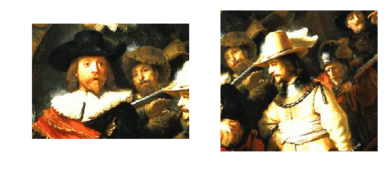
The goal is to automatically make a mosaic out of two images. As an example consider the images nachtwacht1.jpg and nachtwacht2.jpg (see standard images). You have to make a new image that transforms one image to the coordinate system of the other image (using a projective transform) and combine the two images into a larger view of the nachtwacht.

8.3. Projective Transform¶

We start by using Python’s build in functionality for projective transforms. Make sure nachtwacht1.jpg and nachtwacht2.jpg images are somewhere where Python can find them.

In [1]: f1 = plt.imread('images/nachtwacht1.jpg')/255

In [2]: plt.subplot(121); plt.imshow(f1); plt.axis('off');

In [3]: f2 = plt.imread('images/nachtwacht2.jpg')/255

In [4]: plt.subplot(122); plt.imshow(f2); plt.axis('off');

In [5]: plt.show()

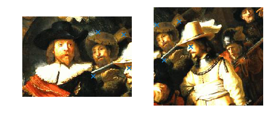
In the left and right image we have selected 4 corresponding points by hand:

# points in left image:
In [6]: xy = np.array([[ 157, 32],
   ...:                [ 211, 37],
   ...:                [ 222,107],
   ...:                [ 147,124]])
   ...: 

# points in right image:
In [7]: xaya = np.array([[  6, 38],
   ...:                  [ 56, 31],
   ...:                  [ 82, 87],
   ...:                  [ 22,118]])
   ...: 

In [8]: plt.subplot(121); plt.imshow(f1); plt.axis('off');

In [9]: plt.scatter(xy[:,0], xy[:,1], marker='x');

In [10]: plt.subplot(122); plt.imshow(f2); plt.axis('off');

In [11]: plt.scatter(xaya[:,0], xaya[:,1], marker='x');

In [12]: plt.show()

From these point correspondences we can calculate the projective transform \(P\) that maps coordinates in the right image (in the xaya array) onto coordinates in the left image (in the array xy).

In the code below we use an OpenCV function to calculate the projection matrix. You are not allowed to use this function!!

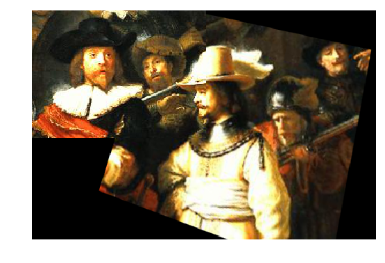
We then warp the right image onto a new image using the projection \(P\). Note that we have selected an output_shape equal to (300, 450) so that the warped image fits in (almost completely).

Then we ‘warp’ the left image to the new image too. In this case we don’t need a warp as we have selected the coordinate axes of the left image as the axes for the stitched image.

In [13]: import cv2

In [14]: from skimage.transform import warp

In [15]: P = cv2.getPerspectiveTransform(xy.astype(np.float32), xaya.astype(np.float32))

In [16]: print(P)
[[  1.01685498e+00   3.12932553e-01  -1.63082057e+02]
 [ -2.17037452e-01   9.92701412e-01   4.39692054e+01]
 [  4.93917724e-04   5.87218302e-04   1.00000000e+00]]

In [17]: f_stitched = warp(f2, P, output_shape=(300,450))

In [18]: M, N = f1.shape[:2]

In [19]: f_stitched[0:M, 0:N, :] = f1

In [20]: plt.imshow(f_stitched); plt.axis('off')
Out[20]: (-0.5, 449.5, 299.5, -0.5)

In [21]: plt.show()

At first sight the result is not too bad but if you look more close you see that the hat of the gentleman in white is ‘torn apart’. This is due to the errors in the corresponding points and therefore the error in the projection matrix.

Exercise

Study the code above and figure out what is done.
Replace the function getPerspectiveTransform with your own code to calculate the projectivity from possibly more then 4 point correspondences (using the SVD trick). This is what you have done in the Lab for the second week. Make sure this code works (even with more than 4 corresponding points: you can point in an image (not when displayed inline in a notebook!) and see the coordinates: just find 2 more corresponding points in left and right image) before you move on.
The shape of the resulting image was manually set in the above code. Note that the top left corner of the right image is not in the stitched result. Can you enlarge the resulting image such that both image are entirely visible in the stitched result?

Unless you can click with subpixel accuracy the combined image undoubtly will show the seams where one image is overlayed on the other image. In order to make image mosaics without noticible seams we need accurate point correspondences and of course we want to automate the entire process. That is where SIFT comes in.

8.4. SIFT¶

The goal is to find the point correspondences in an automated fashion. The scale invariant feature transform (SIFT) is very often used for this purpose. It is invented by David Lowe and reported in the journal article that is perhaps the most often cited article in this field, can be found here.

In [22]: import cv2

In [23]: f = plt.imread('images/nachtwacht1.jpg')

In [24]: fcv2 = f[:,:,::-1] # OpenCV uses BGR ordering of color channels

In [25]: plt.imshow(f);

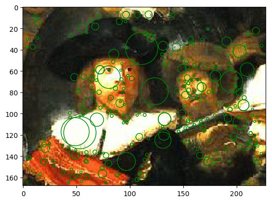
In [26]: sift = cv2.xfeatures2d.SIFT_create()

In [27]: kps, dscs = sift.detectAndCompute(fcv2, mask=None)

In [28]: ax = plt.gca()

In [29]: for kp in kps:
   ....:     ax.add_artist(plt.Circle((kp.pt), kp.size/2, color='green', fill=False))
   ....: 

In [30]: plt.show()

Exercise

In your report you should describe the SIFT in enough detail for your fellow student (who took the vision course but could not attend when SIFT was discussed) to be able to understand it.
Explain in your report why SIFT is scale and rotation invariant.
Extra points for those students that can change the parameters of SIFT from their Python code and experiment with it.

8.5. Matching Descriptors¶

If your run the SIFT detector and descriptor computation on both images you find a set of keypoints and descriptors for both images. To make an initial guess which keypoint in the left image corresponds with a keypoint in the right image only the descriptors are compared. For this you can use the OpenCV bruteforce matcher:

matcher = cv2.BFMatcher()
matches = matcher.match(dscs1,dscs2)

where dscs1 and dscs2 are the descriptors from both images. Read the documentation to learn in what way the matches of the descriptors are encoded.

8.6. RANSAC¶

The possible matching points resulting from the BFMatcher function will undoubtly contain a lot of wrong matches. Therefore we have to decide wich matching points are needed in the estimation of the projective transform. This is where the Ransac algorithm comes in handy.

Exercise

Read the explanation of the Ransac algorithm on Wikipedia and code it in Python/Numpy to be able to estimate a projective transform. OpenCV does provide a function to calculate the projective transforms using RANSAC but you are not allowed to use it!
(For extra points) How many iterations are needed to be reasonably sure to find an optimal solution? You will need some basic knowledge of probability for this.

Advice: first sit down and design your RANSAC algorithm with pen on paper. In case of doubt talk to the assistents.

8.7. Stitching it all together¶

The overall program will look something like:

Calculate the SIFT keypoints and descriptors for both images.
Calculate the matches of the descriptors in the two images.
Use Ransac (and the SVD tric to find a projective transform given corresponding points) to find the projective transform and the set of inliers. Describe this carefully in your report: it really is chicken and egg problem that is tackled in an iterative way. Do not forget to calculate the transform at the end using ALL inliers.

8.8. Report¶

Your report should contain the following sections:

Introduction
Theory. In this section you describe the theory on which your program is based.
- Perspectivities and perspectivity estimation. For this section a short overview of the relevant equations and definitions is enough. In case your week 2 Lab was OK this is a matter of copy and paste, else this is the opportunity to repair the errors.
- SIFT.
  - What are the main steps in the SIFT algorithm
  - Explanation of these steps
  - Illustration of the extrema found in scale space for the nachtwacht images.
- RANSAC. (see a previous section)
Algorithm. A description with pseudo code, or well documented Python code snippets, explaining the entire mosaic construction.
Experiments. The results of applying your code to the nachtwacht and to at least one other set of pictures that you have made yourself (note that all two images of the same scene can be stitched together!).
Conclusions

The total length of the paper should not exceede 6/7 pages (excluding the Python code).