9. Lab: Pinhole Camera¶

9.1. What you will learn¶

What the pinhole camera model is and how it is modelled with a projection in homogeneous coordinates.
How to calibrate the camera, i.e. estimate the camera model parameters using the Direct Linear Transform.

9.2. Camera Calibration¶

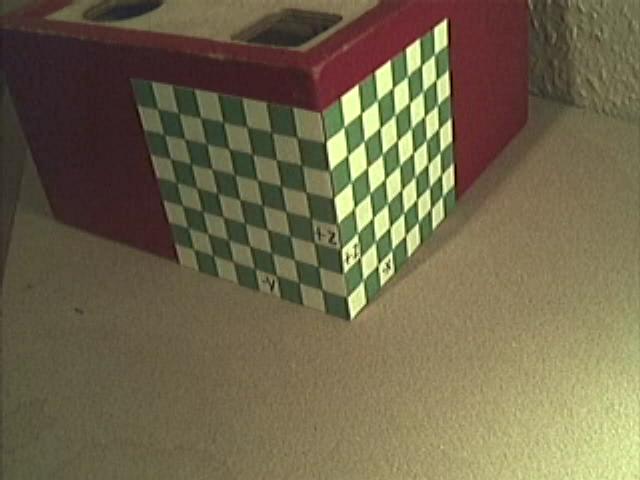
Fig. 9.1 2D projection of a 3D object. On two sides of the box a checker board is drawn. The vertical axis is the positive \(Z\)-direction, the right side checkerboard is the plane \(Y=0\) and the left side checker board is the plane \(X=0\).

The goal of camera calibration is to find the numerical relation between the three dimensional points and the two dimensional points where these are projected. Thus we have to find the camera matrix \(P\) that projects points \((X,Y,Z)\) (in world coordinates) onto the 2D points \((x,y)\) in the image:

\[\hv x \sim P \hv X\]

In this section it is demonstrated that, given the point correspondences \(\hv x_i \leftrightarrow \hv X_i\) for \(i=1,\ldots,n\), we have to solve:

\[\begin{split}\matvec{ccc}{ \hv X_1\T & \v 0\T & -x_1 \hv X_1\T \\ \v 0\T & \hv X_1\T & -y_1 \hv X_1\T \\ \vdots & \vdots & \vdots \\ \hv X_n\T & \v 0\T & -x_n \hv X_n\T \\ \v 0\T & \hv X_n\T & -y_n \hv X_n\T \\ } \v p = \v 0 \\ A \v p = \v 0\end{split}\]

Please note that \(\hv X_i = (X_i\; Y_i\; Z_i\; 1)\T\). The matrix \(A\) given above thus is a matrix in block matrix notation. For your implementation it is easy to first rewrite matrix \(A\) and use the components \(X_i,Y_i\) and \(Z_i\):

\[\begin{split}P &= \matvec{cccc}{ p_{11}& p_{12}& p_{13}& p_{14}\\ p_{21}& p_{22}& p_{23}& p_{24}\\ p_{31}& p_{32}& p_{33}& p_{34} }\\ \v p &= \matvec{cccccccccccc}{ p_{11}& p_{12}& p_{13}& p_{14}& p_{21}& p_{22}& p_{23}& p_{24}& p_{31}& p_{32}& p_{33}& p_{34}}\T\\ A &= \matvec{cccccccccccc}{ X_1 & Y_1 & Z_1 & 1 & 0 & 0 & 0 & 0 & -x_1 X_1& -x_1 Y_1& -x_1 Z_1& -x_1\\ 0 & 0 & 0 & 0 & X_1 & Y_1 & Z_1 & 1 & -y_1 X_1& -y_1 Y_1& -y_1 Z_1& -y_1\\ \vdots&\vdots&\vdots&\vdots&\vdots&\vdots& \vdots& \vdots& \vdots& \vdots& \vdots& \vdots\\ X_n & Y_n & Z_n & 1 & 0 & 0 & 0 & 0 & -x_n X_n& -x_n Y_n& -x_n Z_n& -x_n\\ 0 & 0 & 0 & 0 & X_n & Y_n & Z_n & 1 & -y_n X_n& -y_n Y_n& -y_n Z_n& -y_n }\end{split}\]

To find a null vector of \(A\) we can use the same ‘SVD trick’ that we have used to find the perspecive transform relating 2D points in one image with 2D points in another image (now we are relating 3D points with 2D points).

Given a null vector \(\v p\) we can reshape it into the required camera matrix \(P\).

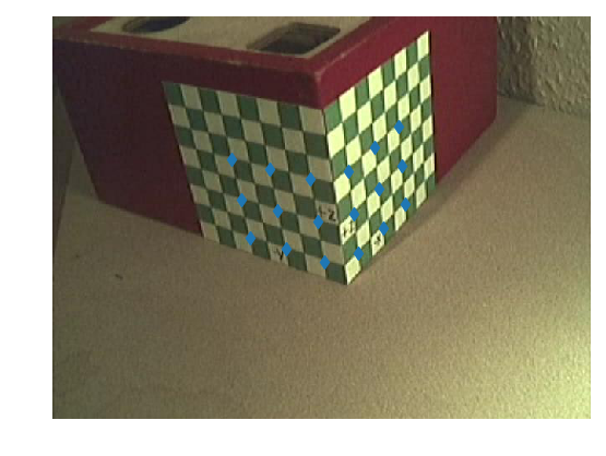
In this exercise we will not discuss (and program) a way to automatically extract points on the calibration object (the box with checker boards that defines the 3D coordinate frame). These points are already indicated (by hand). The matrix xy gives the image coordinates of several points on the left and right checkerboard. Every row in the matrix is a 2D point. The corresponding points in 3D are given as the rows in matrix \(XYZ\).

xy = array([[ 213.1027,  170.0499], [ 258.1908,  181.3219],
            [ 306.41  ,  193.8464], [ 351.498 ,  183.8268],
            [ 382.8092,  155.6468], [ 411.6155,  130.5978],
            [ 223.7485,  218.2691], [ 267.5841,  230.7935],
            [ 314.5509,  244.5705], [ 357.7603,  235.1771],
            [ 387.819 ,  205.1184], [ 415.3728,  178.1908],
            [ 234.3943,  263.9834], [ 276.9775,  277.1341],
            [ 323.318 ,  291.5372], [ 363.3963,  282.1438],
            [ 392.8288,  251.4589], [ 419.1301,  223.9051]])

and

XYZ = array([[0, -5, 5], [0, -3, 5], [0, -1, 5], [-1, 0, 5],
             [-3, 0, 5], [-5, 0, 5], [0, -5, 3], [0, -3, 3],
             [0, -1, 3], [-1, 0, 3], [-3, 0, 3], [-5, 0, 3],
             [0, -5, 1], [0, -3, 1], [0, -1, 1], [-1, 0, 1],
             [-3, 0, 1], [-5, 0, 1]])

In [1]: from pylab import *

In [2]: im = imread("images/calibrationpoints.jpg")

In [3]: imshow(im)
Out[3]: <matplotlib.image.AxesImage at 0x7f1008b2beb8>

In [4]: xy = array([[ 213.1027,  170.0499], [ 258.1908,  181.3219],
   ...:             [ 306.41  ,  193.8464], [ 351.498 ,  183.8268],
   ...:             [ 382.8092,  155.6468], [ 411.6155,  130.5978],
   ...:             [ 223.7485,  218.2691], [ 267.5841,  230.7935],
   ...:             [ 314.5509,  244.5705], [ 357.7603,  235.1771],
   ...:             [ 387.819 ,  205.1184], [ 415.3728,  178.1908],
   ...:             [ 234.3943,  263.9834], [ 276.9775,  277.1341],
   ...:             [ 323.318 ,  291.5372], [ 363.3963,  282.1438],
   ...:             [ 392.8288,  251.4589], [ 419.1301,  223.9051]])
   ...: 

In [5]: plot(xy[:,0],xy[:,1],'d')
Out[5]: [<matplotlib.lines.Line2D at 0x7f0ff1b25b00>]

In [6]: axis('off')
Out[6]: (-0.5, 639.5, 479.5, -0.5)

In [7]: axis('equal')
Out[7]: (-0.5, 639.5, 479.5, -0.5)

Exercises

Write a Python function to calibrate the camera given the corresponding point sets shown above. The result should be matrix \(P\)
The simplest way to test your calibration result is to multiply \(P\) with the homogeneous representation of the 3D calibration points. Obviously the resulting 2D points need to be close to the given 2D points. Calculate the reprojection error as the average error of the 2D points (i.e. the euclidean distance beteen a calibration point in 2D and the projection of the corresponding 3D point).
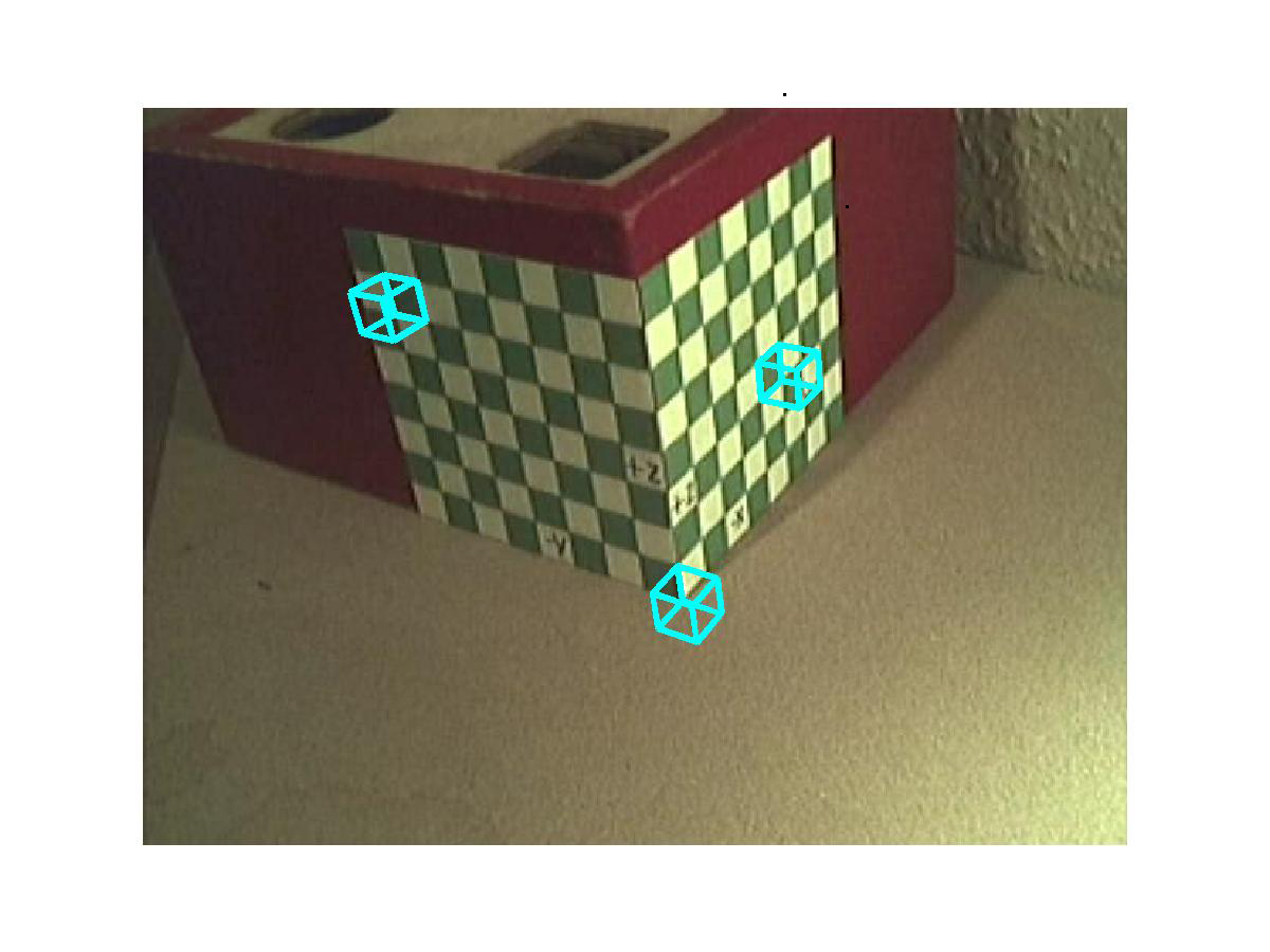
Given the camera matrix \(P\) we can draw 3D objects on the image relative to the 3D coordinate system. In the figure below we have drawn a cube at three different locations.

Write a Python script to draw a unit cube (all sides length 1; i.e. the length of the side of a square on the checkerboards) at a given location in 3D space: drawCube(P, X, Y, Z) where \(P\) is the projection matrix to use and \(X,Y,Z\) is the 3D location.
(for an extra point) Can you make an animation where the cube moves along the circle \(X^2+Y^2=49\) on the table surface (\(Z=0\)). In the lecture series on computer graphics you will learn how to hide the moving cube when it is ‘inside’ the box.