1. Lab Exercise: Installation of Software and Data
1.1. OpenCV
Installing OpenCV is not trivial. You can download binary distributions and install them but it is not always clear that all we need is packaged. For the course we need the module containing the non-free SIFT software.
I am using the anaconda Python distribution. I didn’t install the standard OpenCV but i got a version from binstar:
conda install -c https://conda.binstar.org/menpo opencv3
If all went well you must be able to run the following code:
In [1]: import cv2

In [2]: x = np.arange(128)-64

In [3]: X, Y = np.meshgrid(x,x)

In [4]: f = (100*(np.hypot(X,Y)<32)).astype(np.uint8)

In [5]: plt.clf()

In [6]: plt.imshow(f);

In [7]: plt.gray()

In [8]: sift = cv2.xfeatures2d.SIFT_create()

In [9]: kps, dscs = sift.detectAndCompute(f, mask=None)

In [10]: ax = plt.gca()

In [11]: for kp in kps:
   ....:     ax.add_artist( plt.Circle((kp.pt), kp.size/2, color='green', fill=False))
   ....:

In [12]: plt.show()
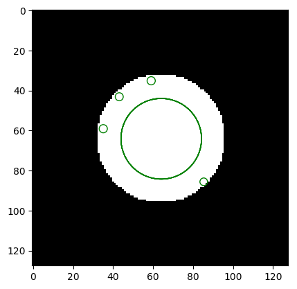
No worries (yet) in case you have a hard time understanding what is done in this code fragment. If you get an image that looks like the one above you have correctly installed OpenCV.
1.2. Standard Images and Data Sets
In the lab exercises you will need some standard data files. All these files are collected in one directory on the web.
1.2.1. Skin Color Data Set
1.2.2. Standard Images
Below are some standard images used a lot in image processing research. The images shown here a small images (\(256\times256\)) which is an advantage when experimenting with code in development.
You can download these images by clicking right on an image.
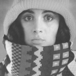
Fig. 1.1 The girl from an advertisement. This image is used a lot by researchers (originally) from Delft University. It is a nice image to use because it contains a lot of details.
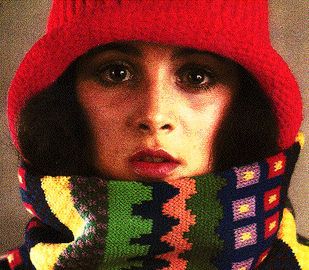
Fig. 1.2 The same girl from the advertisement, this time in color. Note that this is NOT the color version of the same image as shown in gray. Also note that this is scanned copy of a printed image. If you look up close you can see the primary color dots.
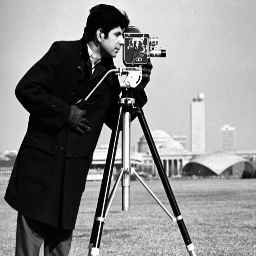
Fig. 1.3 The camera man image. Originally used by researchers in the field of image and video compression.
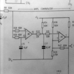
Fig. 1.4 A hand drawn scheme of an electrical circuit. Nowadays most of the technical line drawings are made with computers. In the past most of these drawings were made by hand. Considerable effort has been made to automatically digitize these line drawings into vector graphics formats (i.e. not a simple sampled version of the scanned drawing but a version were lines are recognized and stored as lines).
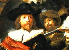
Fig. 1.5 A picture of a small part of the famous ‘Nachtwacht’ painting by Rembrandt van Rijn. Together with the nachtwacht2.jpg image this image is used as an example for building image mosaics.
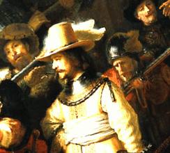
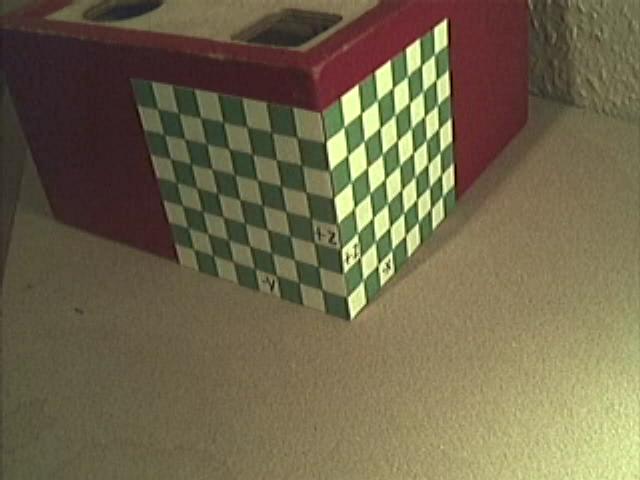
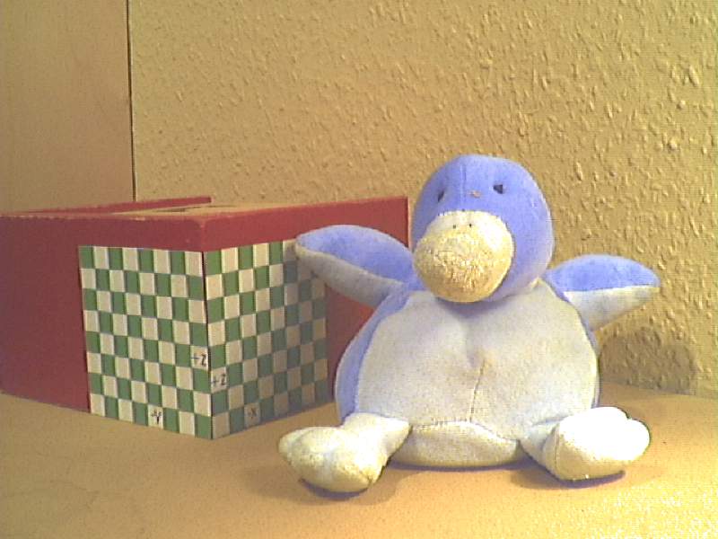
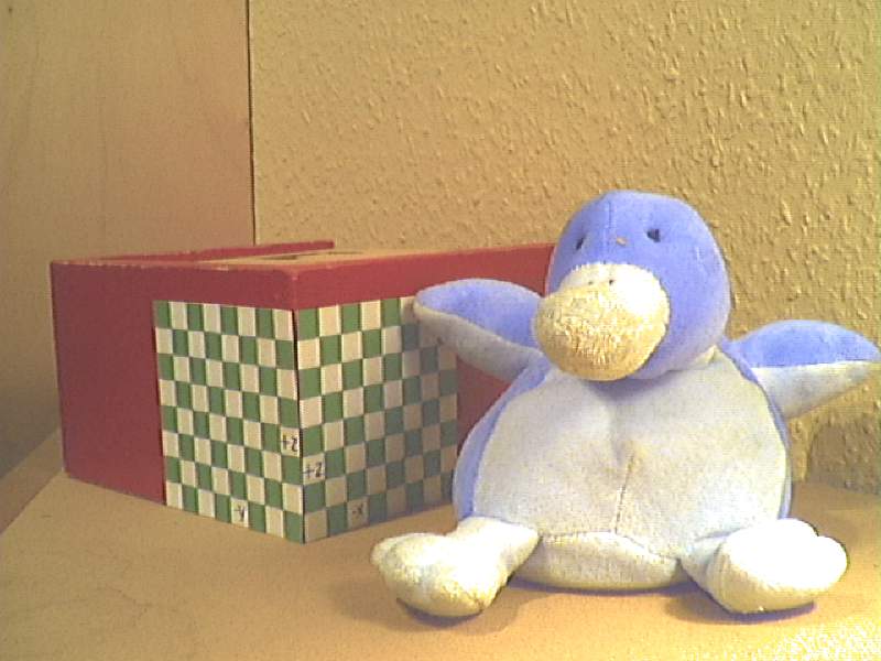
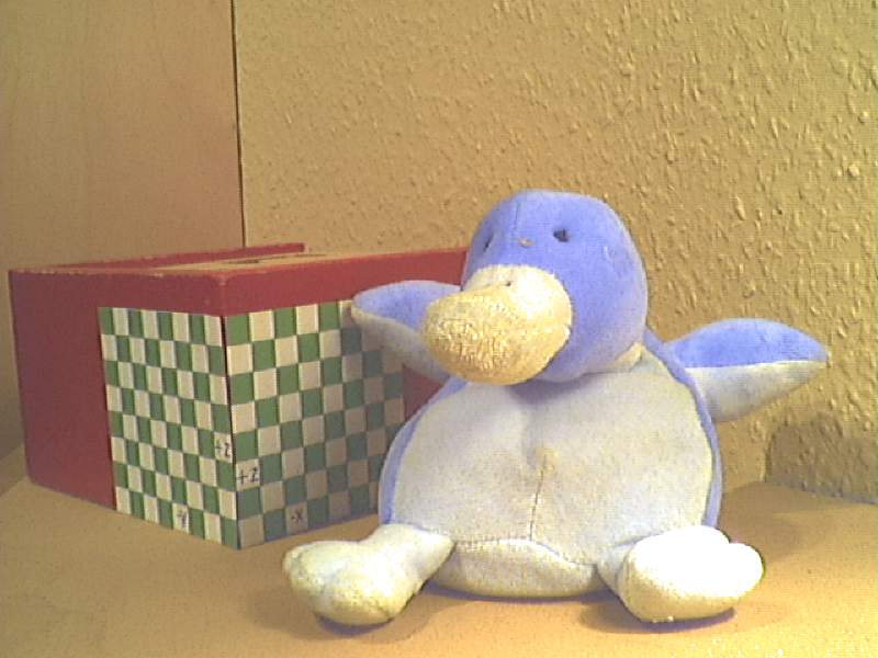
Fig. 1.6 A 2D projection of a 3D object. The checkerboards provide the data to calibrate the camera.
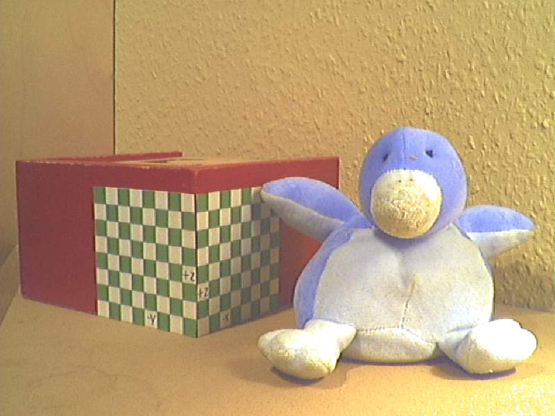
Fig. 1.7 A view of the same calibration object and a cudly animal next to
it. There are several views on this scene available:
/images/view1.jpg, /images/view2.jpg,
/images/view3.jpg, /images/view4.jpg.
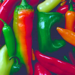
Fig. 1.8 peppers.png. Nice bright colors...
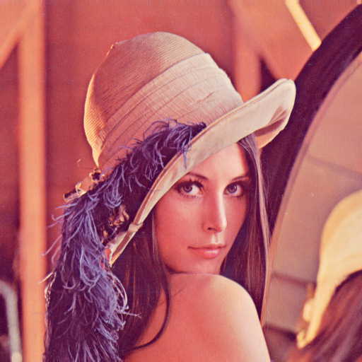
Fig. 1.9 Lena. I am aware of the controversy produced by the use of this image in image processing papers (see Wikipedia). This image is refered to here because of its historic relevance.
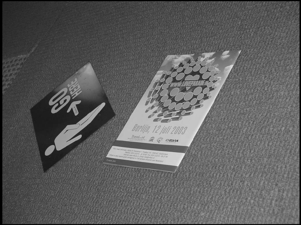
Fig. 1.10 A flyer of size A4 lying on the ground and photographed at an angle from above. The flyer is perspectivily distorted.