6. Lab: Local Structure I
6.1. What you will learn
- To understand the concepts of scale and local structure.
- How to characterize local structure with the Gaussian derivatives.
- What convolutions are.
- How to implement Gaussian image derivatives working on discrete images.
- How to find edges with the Canny Edge Detector.
6.2. Coordinate Axes
In this exercise we are mixing the image indices and graphics coordinates, i.e. we will plot on top of a displayed image.
When we use x and y in this exercise (and xx, X, etc) these are chosen with respect to the graphical axis: x runs from left to right and y runs from top to bottom.
So in case x and y are integer coordinates and we would like to index a numpy array to get the value at that point we have to write F[y,x].
In general when specifying axes for numpy arrays or for parameters to be used in array (image) processing operators we specify them in the order rows then columns.
6.3. Analytical Local Structure
Consider the following function:
Exercise
Calculate analytically the following derivatives of this function: \(f_x\), \(f_y\), \(f_{xx}\), \(f_{xy}\) and \(f_{yy}\) and give the results in your report. Note that \(f_x\) denotes the first order partial derivative in \(x\), etc.
A discrete version of the function \(f\) can be made and visualized in Python with the code:
In [1]: x = np.arange(-100,101); y = np.arange(-100,101);

In [2]: X, Y = np.meshgrid(x,y)

In [3]: A = 1; B = 2; V = 6*np.pi/201; W = 4*np.pi/201;

In [4]: F = A*np.sin(V*X) + B*np.cos(W*Y)

In [5]: plt.clf();

In [6]: plt.imshow(F, cmap=plt.cm.gray, extent=(-100,100,100,-100));

In [7]: plt.show()
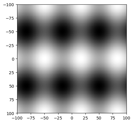
Please make sure you understand what meshgrid does. Display X and Y as images to see what is done. Read the documentation of
imshowto understand theextentargument.Generate the image Fx and Fy, where Fx is the sampled version of the derivative image \(f_x\) that you have calculate analytically before. I.e. sample the function \(f_x\) to get Fx in the same way as in the above piece of code the function \(f\) is sampled to get F. Plot both images in your report.
The values Fx[y,x] and Fy[y,x] are the components of the gradient vector in point (x,y). The following code plots a lot of gradient vectors on top of the original image.
In [8]: Fx = X # this is WRONG

In [9]: Fy = Y # this is WRONG

In [10]: xx = np.arange(-100, 101, 10);

In [11]: yy = np.arange(-100, 101, 10);

In [12]: XX, YY = np.meshgrid(xx, yy);

In [13]: FFx = Fx[::10, ::10]

In [14]: FFy = Fy[::10, ::10]

In [15]: plt.clf();

In [16]: plt.imshow(F, cmap=plt.cm.gray, extent=(-100,100,100,-100), origin='upper');

In [17]: plt.quiver( xx, yy, FFx, FFy, color='red', angles='xy' );

In [18]: plt.show()
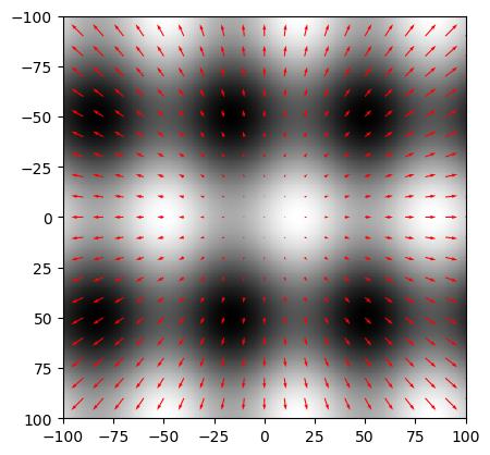
Please note that the quiver plot (plot of gradient vectors) that is calculated and shown is COMPLETELY WRONG... It is your task to fill in the right equations for both derivatives.
In you have the correct derivatives Fx and Fy, the quiver plot should show vector pointing towards the largest increase of gray value.
6.4. Gaussian Convolution
The convolution operator for 2D images is available in the ndimage module of SciPy. The function convolve does the convolution of an image with a 2D kernel (in fact it can do n-dimensional convolutions).
Let F be the discrete image and let W be the kernel then we can
calculate the convolution with G =
convolve(F,W,mode='nearest'). Please read the documentation in case
your kernel is not odd sized as you need to specify the origin of the
kernel then.
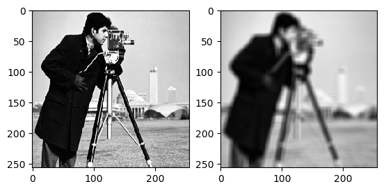
For instance the uniform convolution is calculated as:
In [19]: from scipy.ndimage import convolve;

In [20]: F = plt.imread('images/cameraman.png');

In [21]: W = np.ones((9,9))/81;

In [22]: G = convolve(F,W,mode='nearest');

In [23]: plt.subplot(1,2,1);

In [24]: plt.imshow(F,cmap=plt.cm.gray);

In [25]: plt.subplot(1,2,2);

In [26]: plt.imshow(G,cmap=plt.cm.gray);

In [27]: plt.show()
Exercise
- Write a function
Gauss(s)that returns a 2D sampled Gaussian function with scalesin a numpy array. You should make sure that an appropriate choice is made for the size of the sampling grid. That choice depends on the scale. Furthermore you should make sure that the sum of all kernel values is equal to one. The origin should be in the middle of the array. - In your report you should present a plot of the kernel. In case you have a modern version of matplotlib you might have 3D plotting capabilities (look in the documentation on the web). Else display the array of kernel values for a small value of s (say s=1).
- Given the Gaussian kernel you should be able to do the Gaussian
convolution using
convolve(F,Gauss(s),mode='nearest'). Time the runtime of this function for several values of s (say s=1,2,3,5,7,9,11,15,19) and plot the time versus the scale. Show the plot in your report. What is the order of computational complexity in terms of the scale?
6.5. Separable Gaussian Convolution
The Gaussian function \(G^s(x,y)\) is the unique rotationally symmetric function that can be separated by dimension, i.e. we can write:
where \(G^s_1\) is the one dimensional Gaussian function. The convolution with a separable kernel is easy: *first we convolve along the rows followed by a convolution along the columns.
Let Gauss1(s) be a function call that returns a one dimensional
sampled Gaussian function at given scale s. A convolution along one of
the axis is then done with the specialized function convolve1d(F,
W1, axis=n,mode='nearest')
Exercise
- Write the
Gauss1function. - Calculate the Gaussian convolution using the separability property and time the 2D Gaussian convolution as a function of the scale s. What is the order of computational complexity now?
- (For bonus points) In Matlab the function convolve automagically
checks whether a 2D weight matrix W is separable. Use you
Gaussfunction from a previous exercise to generate a Gaussian kernel. Calculate the SVD of W. What are the singular values? Then what are the 1D convolution kernels that make the 2D convolution separable?
6.6. Gaussian Derivatives
The Gaussian derivatives of an image (function) are calculated by convolving the image with the derivative of a Gaussian function.
Exercise
Show analytically (that is using math) that all derivatives of the 2D Gaussian function are separable functions as well.
Write a function
gD(F, s, iorder, jorder)that returns the Gaussian derivative convolution of image F. The order of differentation isiorderfor the first direction (top to bottom!) andjorderfor the second direction (left to right). Only differentation up to order 2 is needed.Visualize the Gaussian derivative of the cameraman image up to order 2 in your report (i.e. the derivatives \(f\) (zero order), \(f_x\) and \(f_y\) (first order) and \(f_{xx}\), \(f_{xy}\) and \(f_{yy}\) (second order).
Using the
gDfunction you can calculate the discrete first order derivative in x direction withdFx = gD(F, s, 0, 1)
6.7. Comparison of theory and practice
At the start of this exercise you have calculated the derivatives of the function
analytically. You have also sampled this function (for given values of parameters and sampling intervals) to visualize the function as an image.
In this exercise you will have to calculate the derivatives using the
gD function that you have written and compare the results with the
analytical derivatives.
In practice you are mixing derivative calculation with smoothing (the Gaussian convolution). The effect of Gaussian smoothing on this particular function is a multiplication of the sine and cosine function with a factor that is dependent on the frequency. So when comparing your practical derivative result and analytical result you will see that the ratio is constant (well in allmost all of the image).
Exercise
- Compare the analytical first order derivatives in \(x\) and \(y\) of
\(f\) with your discrete implementation, i.e. compare
FxwithdFx = gD(F, 1, 0, 1). - Calculate
Fx/dFx(watch out for points where dFx is zero) and convince yourself that it is nearly constant in every pixel. Where does it deviates from the constant value? - (extra points) Can you explain and calculate the value of the fraction? The easiest way is to use Fourier theory...
6.8. Canny Edge Detector
Exercise
Finding edges in images is often an important first step in image processing applications. Whereas in the past a lot of edge detectors have been suggested, nowadays most often the Canny edge detector is used.
An explanation of the Canny edge detector in terms of local structure as calculated with Gaussian derivatives can be found here.
Implement the Canny edge detector using the
gDfunction that you have implemented in previous sections.The result of the function
E = canny(F, s)should be an imageEwhere the value in a pixel equals the gradient norm (in that pixel) in case it is an edge pixel and zero otherwise.To find the zero crossings in an image you can write a simple function that looks in each 3x3 neighborhood of a pixel whether there are both negative and positive values on opposite sides of the central pixel. This is not a perfect solution but it does the job quite well.
Test your canny function on the camereman image. Show the results in your report for several scales s used in the derivatives calculations.