4.4. Convolutional Neural Network

$\renewcommand{\Cin}{C_{\text{in}}}$ $\newcommand{\Cout}{C_{\text{out}}}$

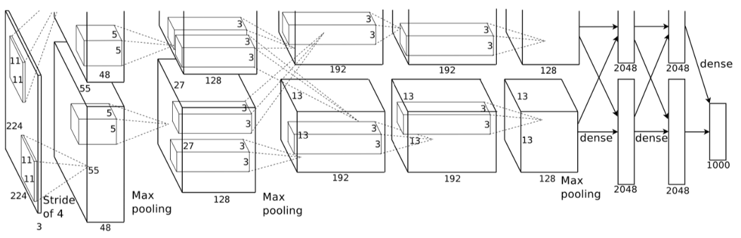
Fig. 4.17 AlexNet.

A CNN follows from the observation that in low level vision the local structure is important. So a fully connected module in such a network is overkill, there are way too many parameters to be learned. Furthermore such a network would be prone to overfitting and not generalize to unseen data. Instead to calculate the value for one pixel in an output image for a processing module in a CNN we consider only a small neighborhood of that point (in an image that is given as input).

Also we would like our processing module to be translation invariant 1, i.e. that all pixels in an image are processed in the same way.

Borrowing the linear weighted sum of input values of the classical fully connected neural network this leads to the convolution 2 as basic processing module in a CNN.

Fig. 4.18 Convolution module in a CNN. The input is a set/block of $\Cin$ images, the output is a set/block of $\Cout$ images. The parameters of such a processing module are the $b_j$’s and the kernels $w_{ij}$’s for $i=1,\ldots,\Cin$ and $j=1,\ldots,\Cout$. Note that the $b_j$’s are scalars and the $w_{ij}$’s are convolutions kernels (typically small with sizes ranging from $3\times3$ to about $11\times11$ and for one processing module typically all of the same size).

Consider the convolutional neural net that started the deep learning era: AlexNet (in Fig. 4.17). The main building block of such a CNN is the convolution module. As input it takes a set of $\Cin$ images $f_i$ ($i=1,\ldots,\Cin$) and produces a set of $\Cout$ images $f_j$ ($j=1,\ldots,\Cout$) according to:

(4.6)\[g_j = b_j + \sum_{i=1}^{\Cin} f_i \ast w_{ij}\]

where $b_j$ is a constant and $w_{ij}$ is one of the $\Cin\Cout$ kernels (all of the same size, at least that is what PyTorch assumes).

Note that the output image sizes ($W_{\text{out}}, H_{\text{out}}$) are not necessarily equal to the input sizes. A quite common choice to deal with the border problem in CNN’s is to restrict the size of the output image such that the convolution kernel fits completely in the image. In that case the size of the output block is dependent on the size of the input block AND on the size of the kernels. Furthermore most frameworks allow for strided convolutions that is conceptually equal to convolution followed by subsampling (and subsampling factor is given by the stride). The interplay of these choices make up for a

As an example the first convolution model in AlexNet (we only consider the lower half of the network) takes in an image block with $W=H=224$ and $\Cin=3$ (a color image) and produces a block of $W=H=55$ and $\Cout=48$. The convolution kernels were all taken to be $11\times11$ kernels. The size of the output block $W=H=55$ comes from combination of the padding, the size of the kernel and the stride (read the PyTorch documentation for the class Conv2d to understand this precisely).

Another method to reduce the spatial size of the images is to insert a max pooling processing module. Max pooling looks like a convolution but instead of taking a (weighted) average of pixel values in a local neighborhood, the maximum value in a local neighborhood is calculated. Again applying a stride for this local maximum filter will reduce the size of the output image.

The linear convolution block associated with the fat arrow in Fig. 4.18 is often followed by a non linear activation function $\eta$. This function is applied element wise to all elements in its input argument. Thus if $g$ is the result of the convolution module than $\eta\aew(g)$.

The back propagation rules for this convolution module associated with the fat arrow in Fig. 4.18 and Eq. (4.6) will be derived in the next subsection. The rules for the activation module and the max pooling module will be taken for granted in these lecture notes 3.

4.4.1. Back Propagation for the Convolution Module

Fig. 4.19 CNN Convolution Processing Module.

For simplicity we concentrate in this section on the convolution processing module depicted in Fig. 4.19 and described by Eq. (4.7) we have left out the bias term. Being an additive term the backpropagation rules for the bias is very easy.

(4.7)\[g_j = \sum_{i=1}^{\Cin} f_i \ast w_{ij}\qquad j=1,\ldots,\Cout\]

As always when deriving back propagation rules for a module we start by assuming that the derivative of the loss with respect to the output is known. In this case we assume that $\partial \ell/\partial g$ is known. Its values (note for every image $g_j$ and for all pixels $f_j(\v y)$ this derivative is represented in with the notation $\partial \ell/\partial g$.

We give the proof for a simplification of the above formula, namely we look at $C_text{in} = C_text{out}=1$ so we have just one convolution to consider:

\[g = f\ast w\]

So now given the derivative of the loss with respect to the output image $g$, what are the derivatives of the loss with respect to the input image $f$ and the weight function (kernel) $w$?

Note that $\partial \ell/\partial g$ is short hand notation for the derivative of the loss with respect to all the pixel values $g(y)$ in the output image. In general the derivative of the loss with respect to all the pixels input image $f$ can be written as:

\[\pfrac{\ell}{f(x)} = \sum_y \pfrac{g(y)}{f(x)} \pfrac{\ell}{g(y)}\]

Calculating the partial derivative of $g(y)$ with respect to $f(x)$ is a bit tricky:

\[\pfrac{g(y)}{f(x)} = \pfrac{}{f(x)} \sum_z f(y-z) w(z)\]

Observe that $z$ ‘runs’ over the entire spatial domain but there is only one value of $z$ such that $y-z=x$ and only for that case the derivative is non zero:

\[\pfrac{g(y)}{f(x)} = w(y-x)\]

note that $y-z=x$ implies that $z=y-x$. Substituting this in the derivative $\partial\ell/\partial g(y)$ gives:

\[\begin{split}\pfrac{\ell}{f(x)} &= \sum_y w(y-x) \pfrac{\ell}{g(y)}\\ &= \sum_y w^m(x-y) \pfrac{\ell}{g(y)}\\ &= \left(w^m \ast \pfrac{\ell}{g}\right)(x)\end{split}\]

Or equivalently:

\[\pfrac{\ell}{f} = w^m \ast \pfrac{\ell}{g}\]

So the forward pass in a convolution module uses a convolution with kernel $w$ maybe surprisingly the backward pass also is a convolution but with the mirrored kernel $w^m$.

Evidently the backpropagation to the derivative of the loss with respect to the kernel is given by:

\[\pfrac{\ell}{w} = f^m \ast \pfrac{\ell}{g}\]

Some observations and words of caution:

In our derivation of the backpropagation rules for the convolution we have implicitly assumed that the images and kernels are defined on the infinite domain $\set Z^2$.
In practice you (well PyTorch really) has to deal with the border problem that arises when considering images and kernels of finite size.
Especially the backpropagation rule for the derivative with respect to the kernel is the correlation of the input image with the derivative $\partial\ell/\partial g$. Both of these functions are entire images but silently only the part of the correlation is calculated that correspond with the pixels in the kernel that is most often in CNN’s quite small (like 3x3 up to 11x11).

The generalization to multiple input channels and multiple output channels is relatively easy as only additions are involved.

4.4.2. A Convolutional Layer in a CNN

One convolutional layer in a CNN is given by:

The convolutions from all the images $f_i$ in the input ‘block” to all the images $g_j$ in the output block:

\[g_j = \sum_{i=1}^{\Cin} f_i \ast w_{ij}\qquad j=1,\ldots,\Cout\]

Adding a bias term $b_j$ a scalar value that is added to all pixels in image $g_j$. It has to be a scalar to make the total operation translation invariant.

Applying a non-linear activation function $\eta$. This function is necessary because without it we would be cascading convolutions leading to convolutions with larger kernels.

Nowadays the classical sigmoid activation function is not often used. The ReLU function is to be preferred to mitigate the vanishing gradient problem.

Fig. 4.20 One Convolutional Layer in a CNN. The input contains $C_\text{in}$ images $f_i$ for $i=1,\ldots,C_\text{in}$, the output contains $C_\text{out}$ images $g_j$ for $j=1,\ldots,C_\text{out}$.

So in total we have the following cascade of function is a convolution layer (see the figure above).

\[g_j = \eta\cdot\left(b_j + \sum_{i=1}^{C_\text{in}} f_i \ast w_{ji}\right)\]

where the activation function $\eta$ is most often the ReLU function:

\[\eta_\text{ReLU}(v) = \max(0, v)\]

In principle you should be able to calculate all the derivatives needed in the backpropagation learning process. But rest assured you don’t have to as PyTorch (or Tensorflow) is quite capable of doing so for you (the derivation as given in the previous section concerning only one convolution should be studied).

4.5. Max Pooling

A typical use of a CNN is to start with a color image (i.e. a block of 3 channels: red, green and blue). Then a convolution is followed by a ReLU activation function. Often some convolution modules are put into sequence. Then the image is subsampled by a factor 2, i.e. each patch of 2x2 pixels is reduced to one pixel. This is done per channel. So for a MaxPool module the number of output channels is the same as the number of input channels. Reducing the 4 values in the 2x2 patch is done using the maximum function.

The rationale behind this non linear function to scale down an image is to have some extra translation invariance.

Because a maxpool module is part of the sequence in the network we should be able to do backpropagation. In case only one pixel in the 2x3 patch is the maximal value the gradient $\partial \ell/\partial g(y)$ is passed on to the pixel at position $x$ in the input image that was the maximum value in this patch. In case several pixels in the 2x2 patch were all the maximal value the gradient would be evenly distributed to these pixels in the input.

Footnotes

1: In the CNN terminology this is often described as equivariance. The word invariance is then preserved for an absolute invariant and equivariance is what in the computer vision community was called relative invariance. In hindsight, equivariance is the better term (but changing all use of invariance in these lecture notes will take some time).
2: In the CNN terminology a convolution is referring to what really is a correlation. Because in the use of CNN’s using a framework like TensorFlow of PyTorch the weight kernels are ‘invisible’ for the programmer the wrong nomenclature not often leads to confusion. For theoretical derivations it is better to use the name convolutions for real convolutions. That is what we will do in these lecture notes.
3: The intention is to make CNN’s more of a central subject in the course. LabExercises that either do not require too expensive laptops (for students) or student access to networked compute servers is essential for this.