5.4. Percentile Filtering

5.4.1. Definition

Show code for figure

import numpy as np
import matplotlib.pyplot as plt
from skimage.io import imread
from scipy.ndimage import percentile_filter
from ipcv.utils.files import ipcv_image_path, get_image_file_path
from skimage.util import random_noise

f = imread(ipcv_image_path('lena.jpg'))[::2, ::2, 1]
f = random_noise(f, mode='s&p')
f0p2 = percentile_filter(f, 20, 5)
f0p5 = percentile_filter(f, 50, 5)
f0p8 = percentile_filter(f, 80, 5)

plt.figure(figsize=(8,8))
plt.subplot(221); plt.imshow(f, cmap=plt.cm.gray); plt.axis('off'); plt.title(r'$f$');
plt.subplot(222); plt.imshow(f0p2, cmap=plt.cm.gray); plt.axis('off'); plt.title(r'$f_{0.2}$');
plt.subplot(223); plt.imshow(f0p8, cmap=plt.cm.gray); plt.axis('off'); plt.title(r'$f_{0.8}$');
plt.subplot(224); plt.imshow(f0p5, cmap=plt.cm.gray); plt.axis('off'); plt.title(r'$f_{0.5}$');
plt.plot()

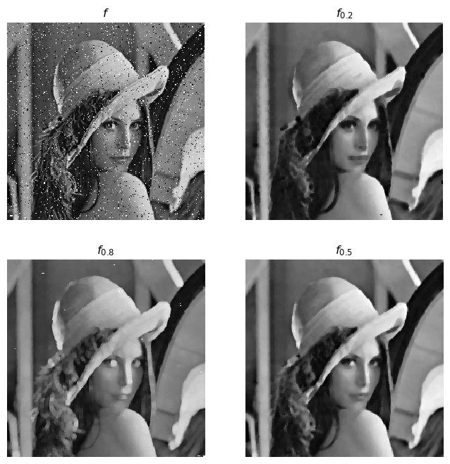
Fig. 5.8 Percentile Filter. The image \(f\) is corrupted with ‘salt & pepper’ noise: random pixels are set to either black (0) or white (1). A Gaussian linear filter cannot really deal with this type of noise (it is meant for additive noise), a percentile filter (especially the median filter \(f_{0.5}\) is doing a great job on this type of noise).

The \(p\)-percentile filter for scalar discrete images is rather simple: in each neighborhood \(\set N\) centered at position \(\v x\) calculate the \(p\)-percentile value of all pixel values in that neighborhood. That percentile value becomes the result of the percentile filter at position \(\v x\). Repeat this for all neighborhoods, i.e. for all points \(\v x\) in the image and you have implemented the percentile filter.

For an introduction to percentiles (and medians, being the \(0.5\)-percentile) see a section in the Mathematical Tools section.

The above simple definition of the percentile/median filter cannot be easily generalized to work with images defined on a continuous domain, where every neighborhood \(\set N(\v x)\) will contain an infinite number of points. Therefore we give at a slightly more complex definition that encompasses both images defined on a continuous domain as well as imaged defined on a discrete domain.

We start by linking percentiles to histograms. Let \(h_f\) be the normalized histogram of the gray values of image \(f\). The \(p\)-percentile then is the minimal value \(t\) such that

\[p = \int_0^t h_f(v) dv = H_f(t)\]

Where \(H_f\) is the cumulative histogram of all gray values in the image \(f\). To restrict the gray values to the neighborhood of \(\v x\), i.e. to all \(f(\v y)\) with \(y\in\set N(\v x)\), we write \(H_{f\bigm|\set N(\v x)}\). Then the percentile filter can be defined as:

Definition 5.17 (Percentile filter)

Let \(f\) be a scalar image and let \(H_{f\bigm| \set N(\v x)}\) be the normalized cumulative histogram of all gray values in the neighborhood \(\set N(\v x)\) then the percentile filter \(\op P_p\) is defined as:

\[(\op P_p f) (\v x) = \inf \left\{ t \bigm| H_{f\bigm|\set N(\v x))}(t) \geq p \right\}\]

The \(p\)-th percentile is thus that value \(t\) such that \(100 p\) percent of the pixels has a value lower then or equal to \(t\).

The \(p=0.5\) percentile is called the median and the corresponding filter is called the median filter.

5.4.2. Algorithms

For an image defined on a discrete grid (a sampled image) the algorithm is very simple. For every neighborhood \(\set N_{\v x}\) in the image, sort all values \(f(\v y)\) (for \(\v y\in\set N_{\v x}\)) in increasing order and pick the \(p\,\#\set N\)-th value in the ordered sequence.

The following code uses the generic filter function from scipy.ndimage to calculate the p-percentile in a \(K\times K\) neighborhood.

from scipy.ndimage import generic_filter

def percentileFilter(f, p, K):
    def pp(vin):
        vout = np.percentile(vin, 100*p)
        return vout
    return generic_filter(f, pp, size=(K,K))

This algorithm is not very efficient. When we move from pixel \((i,j)\) to pixel \((i,j+1)\) the two neighborhoods only differ slightly. Nevertheless all the values in the new neighborhood are sorted from scratch.

The Huang algorithm keeps track of changes in the local histogram while raster scanning the image. When moving from \(\v x_1\) to \(\v x_2\) the values in \(\set N(\v x_1)\setminus \set N(\v x_2)\) must be removed from the histogram and the values in \(\set N(\v x_2) \setminus \set N*\v x_1)\) must be added. Given the histogram and the percentile in point \(\v x_1\), the percentile value in the neighborhood centeren at \(\v x_2\) can be easily calculated.