6.1. Gaussian Convolutions and Derivatives

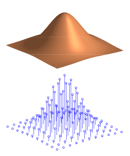
Fig. 6.10 2D Gaussian Function. On top drawn in continuous space and at the bottom as a sampled function.

In a previous chapter we already defined the Gaussian kernel:

Definition 6.2 (Gaussian Kernel)

The 2D Gaussian convolution kernel is defined with:

\[G^s(x,y) = \frac{1}{2\pi s^2}\exp\left(-\frac{x^2+y^2}{2s^2}\right)\]

The size of the local neighborhood is determined by the scale \(s\) of the Gaussian weight function.

Note that the Gaussian function has a value greater than zero on its entire domain. Thus in the convolution sum we theoretically have to use all values in the entire image to calculate the result in every point. This would make for a very slow convolution operator. Fortunately the exponential function for negative arguments approaches zero very quickly and thus we may truncate the function for points far from the origin. It is customary to choose a truncation point at about \(3s\) to \(5s\). In Fig. 6.10 the 2D Gaussian function is shown. Truncated in space in both the continuous space \(\setR^2\) as well as in the discrete space \(\setZ^2\).

6.1.1. Properties of the Gaussian Convolution

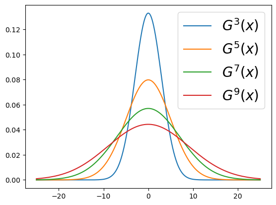
Fig. 6.11 Gaussian Function. for several scales \(s\).

The Gaussian kernel function used in a convolution has some very nice properties.

Theorem 6.3 (Separability of Gaussian Kernel)

The Gaussian kernel is separable:

\[G^s(x,y) = G^s(x) G^s(y)\]

where \(G^s(x)\) and \(G^s(y)\) are Gaussian functions in one variable:

\[G^s(x) = \frac{1}{s\sqrt{2 \pi}} \exp\left( -\frac{x^2}{2 s^2}\right)\]

We have already seen that a separable kernel function leads to a separable convolution (see Section 5.2.6.4). That is why for Gaussian convolutions we show just the 1D functions. In Fig. 6.11 the Gaussian function is shown for several values of \(s\).

Theorem 6.4 (Semi Group of Gaussian Convolutions)

If we take a Gaussian function \(G^s\) and convolve it with another Gaussian function \(G^t\) the result is a third Gaussian function:

\[G^s \ast G^t = G^{\sqrt{s^2+t^2}}\]

Mathematicians refer to such a property with the term semi group (it would be a group in case there would be an ‘inverse Gaussian convolution’).

From a practical point of views this is an important property as it allows the scale space to be built incrementally, i.e. we don’t have to run the convolution \(f_0\ast G^s\) for all values of \(s\). Say we have already calculated \(f^t = f_0\ast G^t\) (with \(t<s\)), then using the associativity and the above property we have:

\[f^s = f^t \ast G^{\sqrt{s^2-t^2}}\]

Note that \(\sqrt{s^2-t^2}<s\) and thus the above convolution will be faster than the convolution \(f_0\ast G^s\).

In the linear scale space view on local structure taking the partial derivatives of image functions is paramount. The Taylor polynomial approximation assumes that we can calculate the partial derivatives of image functions up to order \(N\). But are image functions differentiable? What about discrete sampled images, are these differentiable? These two points are circumvented by not looking for the derivatives of any function (like the ‘zero scale image’ \(f^0\)) but by looking for the derivatives of \(f^0\ast G^s\) with \(s>0\).

Theorem 6.5 (Differentiability)

Let \(f^0\) be the ‘zero scale image’ and let \(f^s=f^0\ast G^s\) be any image from the Gaussian scale space (with \(s>0\)). Then no matter what function \(f_0\) is, the convolution with \(G^s\) will make \(f^s\) into a function that is continuous and infinitely differentiable.

Proof

We leave the proof of continuity to the mathematicians. The differentiability follows directly from Proof 5.11:

\[\partial_{\ldots}(f\ast w) = f \ast \partial_{\ldots} w\]

where \(\partial_{\ldots}\) is any derivative of any order. Applying this for \(w=G^s\) we get:

\[\partial_{\ldots}(f\ast G^s) = f \ast \partial_{\ldots} G^s\]

Note that the Gaussian function is both continuous as well as infinitely many times differentiable. All its derivatives are continuous as well. It is an example of what mathematicians call a smooth function.

Using Gaussian convolutions to construct a scale space thus safely allows us to use many of the mathematical tools we need, like differentiation, when we look at the characterization of local structure.

6.1.2. Derivatives of Sampled Functions

Building a model for local image structure based on calculating derivatives was considered a dangerous thing to do in the early days of image processing. And indeed derivatives are notoriously difficult to estimate for sampled functions. Not only that but when some noise is present in the signal (image in our case) differentiation tends to increase the influence of noise (i.e. high frequencies are increased in amplitude whereas lower frequencies are decreased in amplitude).

Remember the definition of the first order derivative of a function \(f\) in one variable:

\[\frac{d f}{d x}(x) = \lim_{h\downarrow0} \frac{f(x+h)-f(x)}{h}\]

Calculating a derivative requires a limit where the distance between two points (\(x\) and \(x+dx\)) is made smaller and smaller. This of course is not possible directly when we look at sampled images. We then have to use interpolation techniques to come up with an analytical function that fits the samples and whose derivative can be calculated. Three basic ways to estimate the first order derivative for a 1D function are given in the table below:

Name	Equation	Convolution
Left difference	\(F'(x) \approx F(x) - F(x-1)\)	\(F'\approx F\star\{0\;\underline{1}\;-1\}\)
Right difference	\(F'(x) \approx F(x+1) - F(x)\)	\(F'\approx F\star\{1\;\underline{-1}\;0\}\)
Central difference	\(F'(x)\approx(F(x+1)-F(x-1))/2\)	\(F'\approx F\star\frac{1}{2}\{1\;\underline{0}\;-1\}\)

Note that all these ‘derivatives’ are only approximations of the sampling of \(f_x\). They all have their role in numerical math. The first one is the left difference, the second the right difference and the third the central difference. In our study of SIFT we will find use for these derivative operators (but then extended to functions of three dimensions).

In these lecture notes we combine the smoothing, i.e. convolution with a Gaussian function, and taking the derivative. Let \(\partial_\ldots\) denote any derivative we want to calculate of the smoothed image: \(\partial_\ldots(f\ast G^s)\). We may write:

\[\partial_\ldots ( f \ast G^s) = f \ast \partial_\ldots G^s\]

Even if the image \(f\) is unknown (as it always is in practice) and all we have is a sampled image, say \(F\) then we can sample \(\partial G^s\) and use that as a convolution kernel in a discrete convolution.

\[\partial_\ldots (F\star G^s) = F\star \partial_\ldots G^s\]

Note that \(G^s\) is known in analytical form defined on a continuous domain and we can calculate its derivatives analytically.

In Fig. 6.12 the continuous space Gaussian function and its partial derivatives up to order 2 are shown.

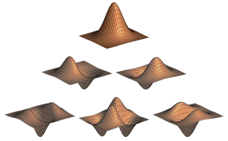
Fig. 6.12 The Gaussian function and its partial derivatives up to order 2. Shown as ‘3D’ plots of 2D functions.

We can also render the Gaussian derivatives as 2D images. These are shown in Fig. 6.13. Note the resemblance with the PCA eigenimages from Fig. 6.8.

Show code for figure

from scipy.ndimage import gaussian_filter

s = 11
N = ceil(3*s).astype(int)
pulse = zeros((2*N+1,2*N+1))
pulse[N,N] = 1


orders = [(1, (0,0)),
          (4, (0,1)),
          (5, (1,0)),
          (7, (0,2)),
          (8, (1,1)),
          (9, (2,0))]
for i, order in orders:
   Gs = gaussian_filter(pulse, s, order)
   mn = Gs.min()
   mx = Gs.max()
   mx = max(abs(mn), abs(mx))
   subplot(3, 3, i)
   imshow(Gs, vmin=-mx, vmax=mx)
   axis('off')

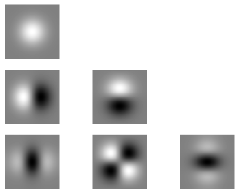
Fig. 6.13 The Gaussian function and its partial derivatives up to order 2. Shown as images (gray at the borders corresponds with zero, white are positve values and black corresponds with negative values).

Note that because \(G^s\) is separable, \(\partial G^s\) is separable as well.

Theorem 6.6 (Separability of Gaussian Derivatives)

All partial derivatives of the Gaussian function are separable:

\[\frac{\partial^{m+n}}{\partial x^m \partial y^n} G^s(x, y) = \left(\pfrac{^m}{x^m} G^s(x) \right)\left(\pfrac{^n}{y^n} G^s(y) \right)\]

This allows for separable convolution algorithms for all Gaussian derivatives. In a LabExercise you have to implement the Gaussian derivative convolutions for the partial derivatives up to order \(2\) (i.e. up to \(m+n=2\)).

As an example in Fig. 6.14 the first order Gaussian derivative of a block function is shown in the continuous domain. In Fig. 6.15 the first order Gaussian derivative of a block function is shown in the discrete domain

Show code for figure

#
# Gayssian (Derivative) Convolutions
#
import numpy as np
import matplotlib.pyplot as plt
from scipy.ndimage import convolve

#plt.ion()
#plt.close('all')

N = 50
x = np.arange(-N//4, N)
f = 1.0 * (x>N//3) * (x<3*N//4) # block function
xx = np.arange(-N//4, N, 0.1)
ff = 1.0 * (xx>N//3) * (xx<3*N//4) # block function


def Gs(x, s):
    return 1/s/np.sqrt(2*np.pi) * np.exp(-x**2 / 2 / s**2)

def Gsx(x, s):
    dx = 1E-3
    return (Gs(x+dx, s)-Gs(x, s))/dx

def Gsxx(x, s):
    dx = 1E-3
    return (Gsx(x+dx, s)-Gsx(x, s))/dx

def sample_kernel(fnc, s, dx):
    N = np.ceil(5*s).astype(int)
    x = np.arange(-N, N+1, dx)
    return fnc(x, s)

kernel = Gsx
s = 2

fig1, axs = plt.subplots(3, 1, sharex=True, figsize=(8,6))
axs[0].plot(xx, ff, label=f"$f$")
axs[0].legend()
axs[1].plot(xx, kernel(xx, s), label=f"$G_x^s$")
axs[1].legend()
W = sample_kernel(kernel, s, 0.1)
gg = convolve(ff, W)
axs[2].plot(xx, gg, label=f"$f\ast G^s_x$")
axs[2].legend()

    


fig2, axs = plt.subplots(3, 1, sharex=True, figsize=(8,6))
axs[0].stem(x, f, label=f"$F$")
axs[0].legend()
axs[1].stem(x, kernel(x, s), label=f"$G^s_x$")
axs[1].legend()
W = sample_kernel(kernel, s, 1)
g = convolve(f, W)
axs[2].stem(x, g, label=f"$F\star G^s_x$")
axs[2].legend()
fig1.savefig('source/images/gDx_block_R2.png')
fig2.savefig('source/images/gDx_block_Z2.png')

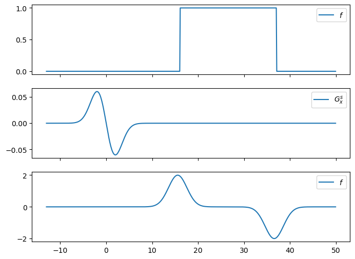
Fig. 6.14 First Order Gaussian Derivative of Block Function.

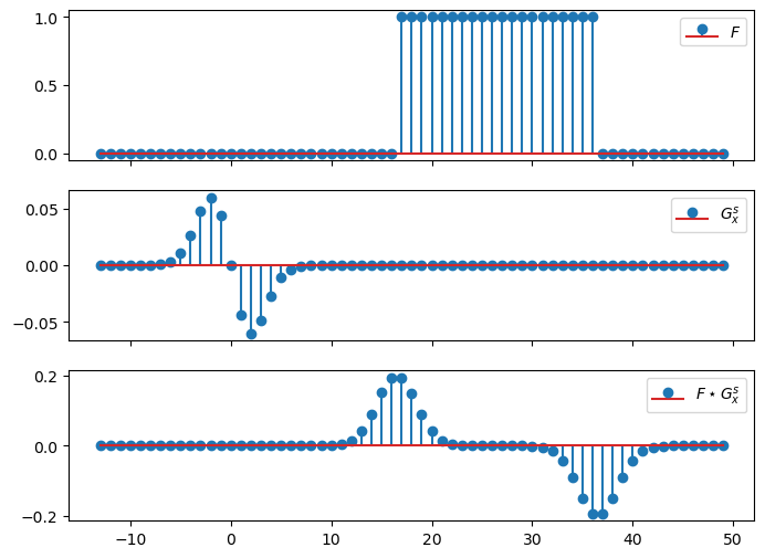
Fig. 6.15 First Order Gaussian Derivative of Block Function.

6.1.3. More about Algorithms for Gaussian Convolutions

There are several ways to implement the Gaussian (derivative) convolutions to work on sampled images:

• Straightforward implementation. This is the direct implementation of the definition of the discrete convolution using the fact that the Gaussian function is seperable and thus the 2D convolution can be implemented by first convolving the image along the rows followed by a convolution along the columns.

  In this straightforward implementation the Gaussian function is sampled on the same grid as the image to be convolved. Although the Gaussian function has an unbounded support (i.e. \(G^s(x)>0\) for all \(x\)) we may ‘cut-off’ the sampled version for values of \(|x|>t\). The value of \(t\) is scale dependent! (this is part of the Lab Exercises).

  It should be evident that for small scale values this straightforward implementation will not be accurate. For, say, \(s<1\) the Gaussian function is restricted to only a few pixels. Such a ‘small’ Gaussian function is really not suited to be sampled on the grid with \(\Delta x\).

• Interpolated Convolution. Instead of bluntly sampling the Gaussian function and calculating the discrete convolution we could first interpolate the discrete image, then calculate the convolution integral and finally sample to obtain the discrete image (this is detailed in the section “From Convolution Integrals to Convolution Sums” in the previous chapter). The interpolated convolution turns out to be equivalent with a discrete convolution with a weight function that is slightly different from the Gaussian (derivative) weight function.

• Convolution using the Fast Fourier Transform. If we first calculate the Fourier Transform of the input image and the convolution kernel the convolution becomes a point wise multiplication. Let the input image be of size \(N\times N\) the spatial implementation is of order \(O(N^2)\) whereas the FFT version is \(O(N\log N)\). This may seem like an important speed up, still the spatial implementation are nowadays more often used.

• Infinite Response Convolution. These are probably the fastest implementations. The gain in speed is obtained because the local neighborhood used is of the same size regardless of the scale of the Gaussian function. Disadvantage of this method is that it is only an approximation and that calculating Gaussian derivatives is troublesome.