3.2.2. Histogram Equalization

Histogram equalization is a point operator such that the histogram of the resultant image is constant. Histogram equalization is often used to correct for varying illumination conditions.

Show code for figure

import numpy as np
import matplotlib.pyplot as plt
from ipcv.ip.pointOps import histogramEqualization
from ipcv.utils.files import ipcv_image_path

plt.figure(figsize=(10,10))
f = plt.imread(ipcv_image_path('cameraman.png'));
print(f.dtype)
g = histogramEqualization(f);
print(g.shape)
plt.subplot(3,2,1); plt.imshow(f); plt.axis('off');
hf, bef = np.histogram(f,bins=20);
plt.subplot(3,2,3); plt.bar(bef[0:-1], hf, width=bef[1]-bef[0] );
plt.subplot(3,2,5); plt.bar(bef[0:-1], np.cumsum(hf), width=bef[1]-bef[0] );

plt.subplot(3,2,2); plt.imshow(g); plt.axis('off');
hg, beg = np.histogram(g,bins=20);
plt.subplot(3,2,4); plt.bar(beg[0:-1], hg, width=beg[1]-beg[0] );
plt.subplot(3,2,6); plt.bar(beg[0:-1], np.cumsum(hg), width=beg[1]-beg[0] );

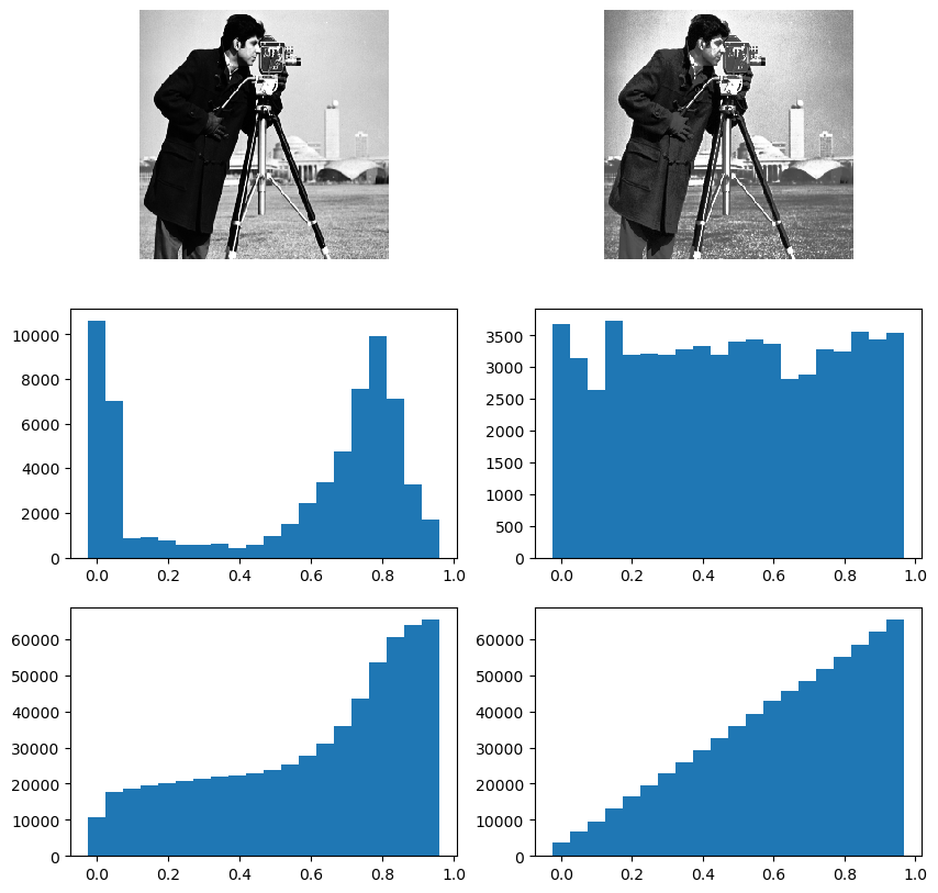
Fig. 3.8 Histogram Equalization. In the first column from top to botton: the original image, its histogram and its cumulative histogram. In the second column the histogram equalized version of the image with its histogram and cumulative histogram.

3.2.2.1. Definition

Let \(f:\set D\rightarrow[0,1]\in\setR\) be a scalar image with histogram (see Section 3.2) \(h_f\). Histogram equalization constructs an image point operator \(\Psi\) such that the resultant image \(\Psi f\) has a constant histogram, in the sense that all scalar values in the resultant image are equally probable. In practice with an image with a finite number of pixels this will not be exactly achievable.

Constructing the transform \(\Psi\) is easy, assuming that it is a point transform, i.e. \((\Psi f)(\v x) = \psi(f(\v x))\) and that the ordering of scalar values is to be preserved, i.e.:

\[v_1 \leq v_2 \Rightarrow \psi(v_1) \leq \psi(v_2)\]

Because the ordering is preserved the p-th percentile of image \(f\) should be equal to the p-th percentile of \(g = \Psi f\). In terms of the cumulative normalized histograms:

\[H_f(v) = H_{g}(\psi(v))\]

Because the histogram of \(g\) is required to be flat (constant) and the image values run from 0 to 1, we have that \(H_{g}(v)=v\), so:

\[\psi(v) = H_f(v)\]

3.2.2.2. Discretization

Now consider the image \(f:\set D\rightarrow[0,255]\in\setZ\). The histogram of \(f\) has at most \(256\) (non empty) bins. The value \(h_f(v)\) for \(v=0,\ldots255\) is the height of the bar in the bar plot of the histogram. Histogram equalization then amounts to moving the bars over the entire range while preserving the order. Bars can be put on top of eachother but the left right relation (order) can not be changed. And of course one bar cannot be split up in two bars. The finite number of different values in the image range thus accounts for the fact that a flat histogram of the result image is not feasible.

3.2.2.3. Practical Use

Histogram equalization is an important image processing operation in practice for the following reason. Consider two images \(f_1\) and \(f_2\) of the same object but taken under two different illumination conditions (say one image taken on a bright and sunny day and the other image taken on a cloudy day). We are interested in how different the scenes in the images are, but cannot simply subtract them. Because of the lighting, there is a non-interesting part to the difference which is explained by an order-preserving mapping, i.e.\(f_2 = \gamma( f_1)\). We should try to discard that first.

It is not hard to prove that the histogram equalized versions of both images are equal: \(\Psi_1 f_1 = \Psi_2 f_2\). Here \(\Psi_1\) and \(\Psi_2\) are the histogram equalizing mappings defined above (these mappings are image dependent, that is why we write the subscript to denote the image).

Histogram equalization thus serves as a preprocessing step in vision systems to compensate for the effect of an unknown change in illumination (grey value scaling). For instance in a face recognition system where images of human faces have to be compared with other images of the same face. Histogram equalization is then a simple first preprocessing step.

3.2.2.4. Code

Using the Numpy function histogram to make histograms and the interp function for linear table interpolation, the code for histogram equalization is simple:

def histogramEqualization(f, bins=100):
    his, be = histogram(f, range=(0,1), bins=bins)
    his = his.astype(float)/sum(his)
    return interp(f, be, hstack((zeros((1)), cumsum(his))))

Here we assume that the original image \(f\) has \([0,1]\in\setR\) as range. We leave it as an exercise to the reader to adapt the code to the case the image has range from \(0\) to \(M\).

3.2.2.5. Exercises

1. Equalization. Let \(f:\set D\rightarrow[0,M]\in\setR\). Give the expression for the function \(\psi\) in this case.

2. Code. In practice scalar images are often 8, 10 or 12 bit per pixel. In such cases it is unnescessary to first convert the image into a floating point image (with 32 or even 64 bits per pixel), you would like a histogram equalization algorithm to work on the integer representation instead of a real valued representation. Write a program to do just that.

   Hint: an often used way to do this is to work with a look-up table. For each possible scalar value v you calculate the histogram equalized value (and you may use floating point values here) and store the result in an array, say HE. In Numpy the actual table lookup then is as simple as HE[image] where image is the original image array. Note that we are using a nice indexing feature of Numpy arrays: the shape of the index (the image in this case) determines the shape of the indexing operation.

   Please note that the imread function from matplotlib always returns a floating point representation of an image even it was stored in the file in an 8 bit per pixel format.

   To read the file and preserve the datatype as stored on disk is to use imread from skimage.

   from skimage.io import imread as skimread f = skimread(‘data/cameraman.png’) print(f.dtype)

3. Practical Use. Make several (at least 4) pictures of the same scene/object from different points of view. Most likely the overall intensity distribution in the images is not equal due to the automatic lighting correction in your camera. Use histogram equalization to correct for this and comment on whether it does the intended job. In your notebook you have to show a 2 x n ‘matrix’ of images, in the top row the original images and in the bottom row the equalized images.

   Your camera probably makes color images. Equalization as discussed works on gray value images (black and white images). You can use the function rgb2gray from sklearn.color to make black-and-white images out of your color images.

   Note: for bonus points. A simple way to use equalization on color images (and have a color image as the result) is to first convert the color image to a colorspace that explicitly encodes the luminance (the gray value) and the color component. One example is the function rgb2hsv from sklearn.color. HSV stands for Hue, Saturation and Value, where value is the gray value component. Equalization of color images then amounts to: convert a rgb image into a hsv image, then equalize the v component and then convert the new hsv image back to rgb (with hsv2rgb).

4. Interpolation. The function interp is actually a simple interpolator for a one dimensional function. Let xs be the array of sample x-values and F the array of sample function values of a function in these sample points. Then interp(x,xs,F) calculates the interpolated function value for given x using a simple linear interpolation scheme. Let the number of samples in xs (and thus in F) be equal to \(N\) what is the order of complexity for an efficient algorithm to implement the interp function? Note: you may only assume that the sample x values in xs are ordered, i.e. that all(diff(xs))>0 is True.