7.3. Sampling Linear Scale-Space

\[\newcommand{\nscales}{n_\text{scales}} \newcommand{\smax}{s_\text{max}}\]

Most of what we have done in the chapter up to now has been formulated for images in the continuous domain. And it is due to our use of the Gaussian derivatives that this is even true for everything involving derivatives. In practice working with discrete (i.e. sampled images), when using the simple strategy of discretizing the convolution operation by sampling the kernel function as well, we are doing ok in case the scale of the Gaussian filter involved in the Gaussian derivative is greater than ome.

So we are used to deal with sampled images in practice. Sampling an image in the spatial domain is invariably done using a regular, most often square, grid of sample points. But what about sampling a scale space? Let \(F^{s_0}\) be the sampled version of the image we start with in constructing a scale space, i.e.

\[F^{s_0}(\v k) = f^{s_0}(B \v k)\]

then the image \(F^s\) at scale \(s\) is calculated from \(F^{s_0}\) as:

\[F^s(\v k) = F(\v k, s) = \left( F^{s_0} \star G^\sqrt{s^2-s_0^2}\right)(\v k)\]

To store and process the scale space we have to decide for which scales \(s\) to calculate and store the convolutions. You might be tempted to use a equidistant sampling of the scale as well. But that would require a dense sampling of the scale and because scale tends to be of interest over several orders of magnitude (scales ranging from tenths to hundreds are not uncommon) that would require a tremendous number of scales to process. And it is not needed. You can try it for yourself and for instance compare images at scale \(s=1\) and \(s=2\). The increase in scale is quite noticable in that case. But comparing \(s=100\) with \(s=101\) shows hardly any difference at all. It is better to sample scale equidistantly on a logarithmic scale axis.

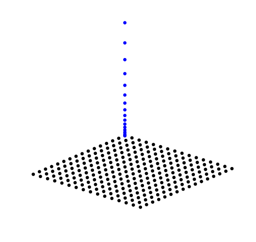
Fig. 7.7 Sampling Scale Space. To avoid visual clutter we have only shown the sample points in space for scale \(s_0\) and the scale samples for \(\v k=\v 0\).

Definition 7.7 (Logarithmic Scale Sampling)

The scale in scale space is sampled logarithmically. If \(s_0\) is the first scale (often the scale of the image that was obtained with a camera) then the scales are:

\[s_i = \alpha^i s_0\]

for \(i=0,\ldots,\nscales-1\) where \(\smax=s_{\nscales-1} = \alpha^{\nscales-1} s_0\) defines the maximal scale we are interested in. The constant \(\alpha\) defines the (multiplicative) step size along the scale axis.

As a rule of thumb the scale factor \(\alpha\) should be somewhere in the region \(1<\alpha\leq2\). With the extreme value \(\alpha=2\) the scale doubles with every scale sample. Although that is nice from a computational point of view (see the subsection on Burt pyramids) we often opt for a smaller \(\alpha\) in order not to miss important features in scale space (e.g. when looking for the exact localization of blobs in scale space).

7.3.1. Direct versus Incremental Calculation

Let our goal be to make a scale scape from initial image \(F^{s_0}\) where where take \(s_0=0.5\). In that case the receptive fields of the samples just overlap. Let the largest scale we want to represent in the scale space be \(s_\text{max}\) and we wish to have \(n_\text{scales}\) scales starting at \(s_0\) and ending at \(s_S=s_\text{max}\) then the \(\alpha\) value follows from that:

\[\alpha = \left(\frac{\smax}{s_0}\right)^\frac{1}{\nscales-1}\]

The images \(F^{s_i}\) are calculated as:

\[F^{s_i} = F^{s_0} \star G^{s_0 \sqrt{\alpha^{2i}-1}}\]

for \(i=1,\ldots,\nscales-1\). Note that \(F^{s_0}\) is the original image and needs no convolution. We will call this the direct calculation of the scale space.

Show code for figure

import numpy as np
import matplotlib.pyplot as plt
from scipy.ndimage import gaussian_filter as gD


def make_scale_space_direct(f, s_0, s_max, n_scales):
    alpha = (s_max / s_0)**(1 / (n_scales - 1))
    scales = s_0 * alpha**np.arange(n_scales)
    diff_scales_from_s0 = np.sqrt(scales[1:]**2 - s_0**2)

    fs = np.empty((n_scales, *f.shape))
    fs[0] = f.copy()

    for i, s in enumerate(diff_scales_from_s0):
        fs[i + 1] = gD(f, s)

    return fs, scales


def make_scale_space_incremental(f, s_0, s_max, n_scales):
    alpha = (s_max / s_0)**(1 / (n_scales - 1))
    scales = s_0 * alpha**np.arange(n_scales)
    diff_scales_from_si = np.sqrt(scales[1:]**2 - scales[:-1]**2)

    fs = np.empty((n_scales, *f.shape))
    fs[0] = f.copy()

    for i, s in enumerate(diff_scales_from_si):
        fs[i + 1] = gD(fs[i], s)

    return fs, scales


def make_scale_space_octaves(f, O, k, s0):
    n = O * k
    alpha = 2 ** (1 / k)
    scales = s0 * alpha ** np.arange(n)
    conv_scales_from_s0 = s0 * np.sqrt(alpha ** (2 * np.arange(n)) - 1)

    fs = np.empty((n, *f.shape))
    fs[0] = f.copy()

    for i, s in enumerate(conv_scales_from_s0[1:]):
        fs[i + 1] = gD(f, s)

    return fs, scales


plt.close('all')

try:
    f = plt.imread('../../source/images/voc21.jpg')
except FileNotFoundError:
    f = plt.imread('source/images/voc21.jpg')

g = f[38:348, 156:400, 1] / 255

n_scales = 8
s0 = 0.5
s_max = 32
fs_direct, scales = make_scale_space_direct(g, s0, s_max, n_scales)

fig_scsp_direct, axs = plt.subplots(1, n_scales, figsize=(n_scales, 2))
n = n_scales

for i, s in enumerate(scales):
    axs[i].imshow(fs_direct[i], cmap=plt.cm.gray)
    axs[i].axis('off')
    axs[i].set_title(f"{s:2.2f}")

    plt.tight_layout()


fs_incremental, scales = make_scale_space_incremental(g, s0, s_max, n_scales)

fig_scsp_incremental, axs = plt.subplots(2, n_scales, figsize=(n_scales, 4))
n = n_scales

for i, s in enumerate(scales):
    axs[0, i].imshow(fs_incremental[i], cmap=plt.cm.gray)
    axs[0, i].axis('off')
    axs[0, i].set_title(f"{s:2.2f}")

    axs[1, i].imshow(fs_direct[i]-fs_incremental[i], cmap=plt.cm.gray)
    axs[1, i].axis('off')
    axs[1, i].set_title(f"{(np.abs(fs_direct[i]-fs_incremental[i])).max():2.1E}")
    plt.tight_layout()
fig_scsp_direct.savefig('source/images/scsp_voc21.png')

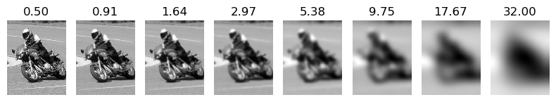
Fig. 7.8 Direct calculation of a scale space. All scales \(s>s_0=0.5\) are calculated as \(F^{s_0} \star G^{s_0 \sqrt{\alpha^{2i}-1}}\). The scale \(s_i\) is printed above the images.

Instead of the direct calculation of scale space we may take the image at scale \(s_i\) to calculate the image at scale \(s_{i+1}\):

\[F^{s_{i+1}} = F^{s_i} \star G^{\sqrt{s_{i+1}^2 - s_i^2}}\]

This is called the incremental calculation of scale space. The advantage is that incremental calculation is more efficient (faster) as the scales in convolutions are smaller. A disadvantage is that the Gaussian convolution is less accurate for smaller scales. As a rule of thumb we do need a scale for the convolution kernel greater than around 0.7.

Show code for figure

# for code see previous figure
fig_scsp_incremental.savefig('source/images/scsp_voc21_incremental.png')

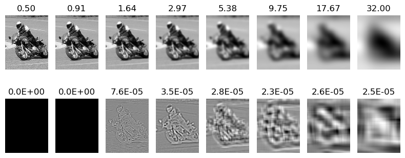
Fig. 7.9 Incremental calculation of a scale space. In the first row the scale space images calculated incrementally. On the second row the difference images for all scales are shown (note that the very small differences are displayes over the entire dynamic range of the display, and therefore look larger than they are). In the first row the scale is printed at the top of an image, In the bottom row the maximal absulte difference of the images at scale \(s_i\) calculated directly and incrementally.

From the figure it is clear that the differences are very (neglibly) small. So where possible an incremental calculation is called for. Note that in case we are calculating the scale space of a derivative we must be more careful.

7.3.2. Pyramids

When constructing a scale space we are smoothing images. After smoothing an image we need less pixels to represent the image faithfully. The exact understanding of this fact requires knowledge of the sampling theorem which falls outside the scope of this lecture series. But you can imagine that when we smooth out local variations in an image we can subsample the image without loosing too much information.

As a rule of thumb, which is useable when using Gaussian smoothing, we may subsample an image with a factor of 2 (in both directions) when the scale of smoothing has doubled.

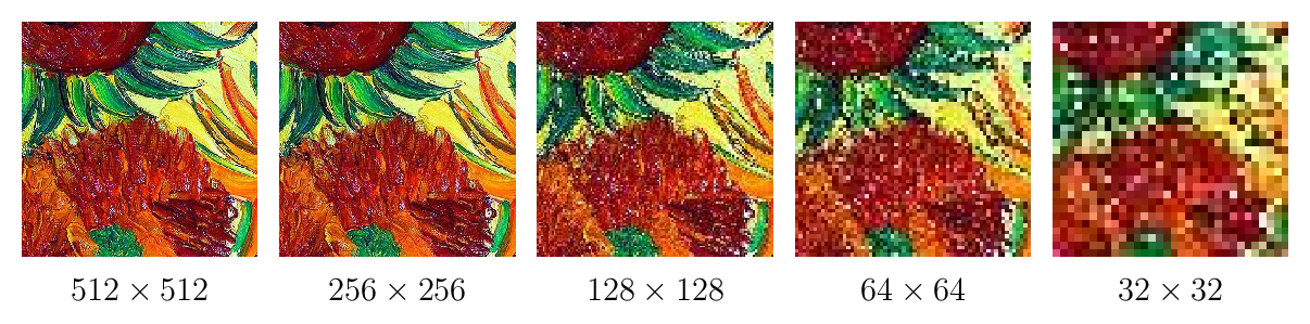
Fig. 7.10 Subsampling Images WITHOUT Smoothing.

Carefully note that smooting is a prerequisite for subsampling. In Fig. 7.10 we show an image and its subsampling without smoothing. It should be evident from these images that subsampling without smoothing leads to artefacts in the image (the ‘noise’ in the subsampled images for the smaller sizes Fig. 7.10).

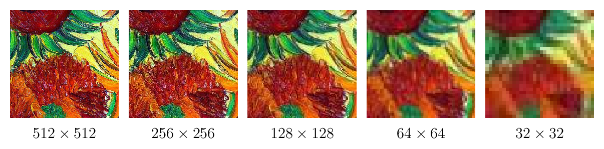
Fig. 7.11 Subsampling Images WITH Smoothing. From left to right \(F^{s_0}\) at full resolution, \(F^{2s_0}\) at half resolution, \(F^{4s_0}\) at a fourth of the original resolution, \(F^{8s_0}\) at an eight of the original resolution and finally \(F^{s_0}\) at an sixteenth of the original resolution. Note that there are no subsampling artefacts.

In Fig. 7.11 the same sequence of subsampled images is shown but this time presmoothing is used. It is obvious that in this way no artefacts (aliasing in signal processing jargon) is introduced.

In this figures in this subsection we have only shown subsampling steps with a factor of two. This is not actually needed, after smoothing and having calculated \(F^{\alpha s_0}\) we can subsample with a factor \(\alpha\). Subsampling with a fraction that is not equal to a power of two is more difficult and often involves some kind of interpolation. It is therefore not often used.

7.3.2.1. Burt Pyramid

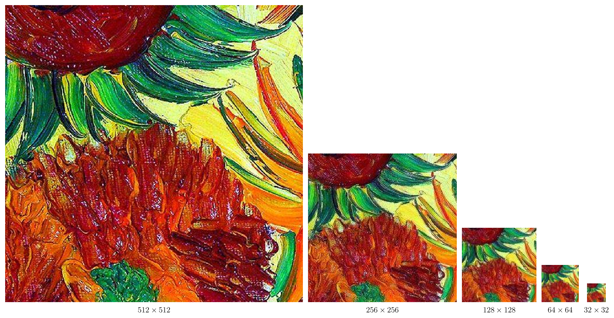
Fig. 7.12 Burt Pyramid.

The sequence of images as shown in Fig. 7.11 is what is known as a Burt pyramid. In Fig. 7.12 the same images are shown in sizes that reflect their resolution.

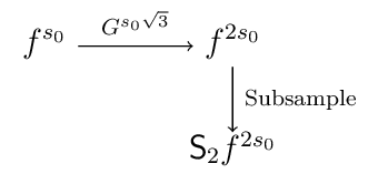
The advantage of using an image pyramid is that a neighborhood of size \(s\) in an image corresponds with a neighborhood of size \(s/2\) in the image at half resolution. Let \(\op{S}_\alpha\) denote the subsampling operator with a factor \(\alpha\), i.e. \(\op S_2 F\) is the subsampling with factor 2 of image \(F\). Then we have that:

\[\op S_\alpha (F \ast G^s) \approx \op S_\alpha F \ast G^{\frac{s}{\alpha}}\]

It is only approximately true as subsampling will induce some loss of information (because ideal low pass filters and ideal band limited signals do not exist, again you will need to learn about signal processing to be able to prove this).

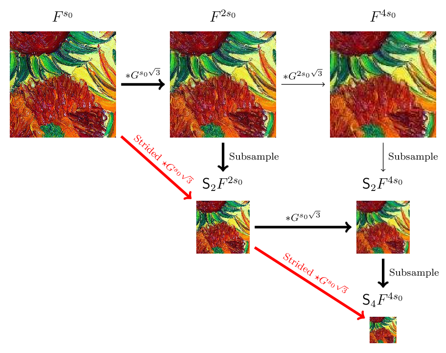
Fig. 7.13 Burt Pyramid. Shown are two subsampling steps in a Burt pyramid.

In Fig. 7.13 two subsampling steps in a Burt pyramid are shown. On the first row the three images \(F^{s_0}\), \(F^{ss_0}\) and \(F^{4s_0}\) are shown and the scales of the Gaussian convolutions needed in the incremental convolutions. Note that the size of the incremental convolution doubles. Instead of the convolution to calculate \(F^{4s_0}\) from \(F^{2s_0}\), we could start with \(\op S_2 F^{2s_0}\). Due to the halving of the resulotion we can halve the size of the Gaussian kernel as well and calculate \(\op S_2 F^{4s_0}\). Note that now the scale of the Gaussian kernel in the convolution is the same as for the first step when building the pyramid. In the construction of the Burt pyramid we thus need only one scale for the Gaussian convolution. That convolution can thus be highly optimed for speed.

The fat black arrows indicate the path that is followed in constructing the pyramid. In practice we can take a shortcut. We don’t need to calculate the convolutions at the resolution of the input image. We can just calculate the convolution sum only for those points that are used in the subsequent subsampling process. In the jargon nowadays used in deep learning this is called a strided convolution. These ‘shortcuts’ are indicated with the red fat arrows in Fig. 7.13.

7.3.2.2. Lowe Pyramid

Although the Burt pyramid is very space (and time) efficient it is not an accurate scale space representation. For instance when looking for blobs in an image (of unknown size) the Burt pyramid will fail to detect blobs with sizes inbetween the scales that are sampled (\(2^i s_0\)). For accurate detection of blobs of all sizes we need an \(\alpha\) value less than 2.

One of the original contributions of Lowe in his SIFT paper is his use of a Burt like pyramid with an \(1<\alpha<2\). He picks an \(\alpha\) value such that \(\alpha^k\) is 2 for some integer value \(k\), i.e. \(\alpha=\sqrt[k]{2}\). Each interval of scales:

\[2^n s_0 \leq s < 2^{n+1} s_0\]

is called an octave. The scales in a scale space starting at scale \(s_0\) then are \(s_i = \alpha^i s_0 = (\sqrt[k]{2})^i s_0\). Take \(k=3\) then the scales in the first three octaves are:

\[\underbrace{s_0\quad \alpha s_0\quad \alpha^2 s_0}_ {\text{first octave}}\quad \underbrace{2 s_0\quad 2 \alpha s_0\quad 2 \alpha^2 s_0}_ {\text{second octave}}\quad \underbrace{4 s_0\quad 4 \alpha s_0\quad 4 \alpha^2 s_0}_ {\text{third octave}}\]

Whereas in the Burt pyramid one stage for doubling the scale is given as:

for the Lowe pyramid (with \(k=3\)) we have:

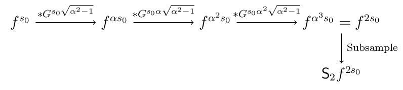
Note that the scales for the Gaussian convolutions in every stage of the pyramid construction are the same. Also note that if we would like to start the scale space at \(s_0\) (which is often assumed to be 0.5) the scales we need in the Burt pyramid for \(k=3\) are:

\[\begin{split}s_0 \sqrt{\alpha^2-1} &\approx 0.38\\ s_0 \alpha \sqrt{\alpha^2-1} &\approx 0.48 \\ s_0 \alpha^2\sqrt{\alpha^2-1} &\approx 0.61\end{split}\]

Gaussian convolution at these scales are numerically hard to implement and because they necessariy involve some interpolation and thus smoothing they are inaccurate. Therefore Lowe introduced a base scale \(s_b=1.6\) which serves a new value for the scale of the image we start with. The image at scale \(s_0\) is first convolved with a Gaussian kernel of scale \(\sqrt{s_b^2 - s_0^2}\) and this image is from then on taken as the first image in the Lowe scale space pyramid.

The scales then needed to construct the images in one octave (again with \(k=3\)) are:

\[\begin{split}s_b \sqrt{\alpha^2-1} &\approx 1.23\\ s_b \alpha \sqrt{\alpha^2-1} &\approx 1.55 \\ s_b \alpha^2\sqrt{\alpha^2-1} &\approx 1.95\end{split}\]

These scales are large enough to allow for a straightforward sampling of the Gaussian kernel to be used in a discrete convolution.