3.2. Histogram Based Image Operations
Consider a unary point operator. Every pixel value in the image is replaced with a new value. What could be the practical use of such a simple operation? In fact there are many uses and most of them are based on the analysis of what pixel values are present in the image. Computing the histogram provides this information compactly.
Here we consider scalar images \(f:\set D\rightarrow \set R\) with range \(\set R = [0,1]\in\setR\). Let \(\phi\) be a function from \([0,1]\in\setR\) to \([0,1]\in\setR\) then we define the monadic point operator:
A monadic point operator thus changes the pixel value \(f(\v x)\) independent of the position \(\v x\) and independent of all other pixel values in the neighborhood.
A nice way to interpret and analyze a monadic point operator is to consider what the operator does with the image histogram. Or the other way round: we may specify desired properties of the histogram of the resulting image and see what point operator results in a image whose histogram has the specified properties.
An image histogram summarizes which values \(v=f(\v x)\) are present in an image \(f\). The histogram function \(h_f(v)\) is proportional to the number of pixels with gray value \(v\). For a discretized and sampled image where the gray values are integers, say in the range from 0 to 255, the histogram counts the number of pixels with a particular value. For an image with real valued gray values in the range from say 0 to 1 we have to divide the range of possible values into discrete bins. Bins are most often taken of equal size. Note that for a sampled image (with a finite number of pixels) we cannot take the bin size too small because then many bins will be empty. Selecting too few bins will not correctly represent the distribution of the gray values in the image.
In Fig. 3.6 the histogram of several images are shown with different choices for the bin size. Look at the code to see how to calculate a histogram of an image.
Show code
 1import numpy as np
 2import matplotlib.pyplot as plt
 3from skimage.color import rgb2gray
 4
 5
 6histsizes = [16, 32, 64]
 7Nhists = len(histsizes)
 8imagenames = ['trui.png', 'cameraman.png', 'rice.png']
 9Nims = len(imagenames)
10fig, axs = plt.subplots(Nhists+1, Nims, sharey='row', figsize=(6,4))
11for i, name in enumerate(imagenames):
12    impath = 'python/data/images/'+imagenames[i]
13    im = plt.imread(impath)
14    if len(im.shape)>2: im = rgb2gray(im)
15    axs[0,i].imshow(im, cmap=plt.cm.gray)
16    axs[0,i].axis('off')
17    for j, nbins in enumerate(histsizes):
18        h, be = np.histogram(im, bins=histsizes[j], range=[0,1], density=True)
19        axs[j+1,i].bar(be[:-1], h, width=be[1]-be[0])
20
21fig.set_size_inches(6, 8)
22fig.tight_layout()
23plt.savefig('source/images/image_histograms.png')
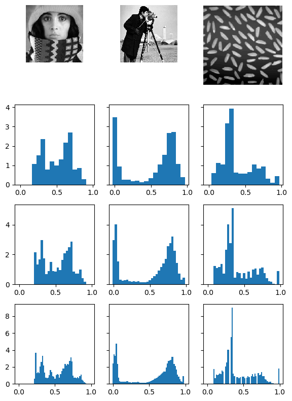
Fig. 3.6 Image histograms. On the first row three gray scale images are plotted. On the rows beneath the images the histograms of those of images are shown using 16, 32 and 64 bins.
The cumulative image histogram \(H_f(v)\) of a sampled image \(f\) counts the number of pixels with a gray value less than or equal to \(v\).
Note: an image histogram can be interpreted as the estimator for the probability mass (or density) function of a distribution of which we have as many examples as there are pixels in the image. The cumulative histogram then is the estimation of the cumulative distribution function.
To stress this observation the image histogram is often calculated as the normalized histogram such that for a sampled image the sum of all bin values \(h_f(v)\) equals 1.
Plotting an image histogram immediately reveals whether the whole range of possible gray values is used in the image. Doing so is most often a desirable property: missing large gray values and the images might be too dark, missing low values and the image might be too light. Contrast stretching is a technique to construct a new image that uses the whole range of all possible gray values.
Histogram equalization applies a monadic point operator to an image such that the resulting image has an histogram that is constant. Equalization is often used to normalize the gray values (or luminance in color images) to be invariant to changes in illumination conditions.
In many practical applications of image processing the imaging conditions are such that the objects of interest can be seperated from the background based on the gray values. E.g. low gray values corresponds with objects and high gray values with the background (think of a gray value scan of a piece of paper with text in black ink). Threshold is the simple operator \(f>=t\) where \(f\) is the image and \(t\) is the threshold value. We will look at one method to calculate \(t\) based on the histogram of \(f\).