3.2.3. Thresholding

Visual inspection of a lot of images reveals that the objects of interests (the coins in the image below) have a gray value that is different from the background. In these cases the histogram will often show a bimodal distribution.

Show code for figure

import numpy as np
import matplotlib.pyplot as plt
from ipcv.utils.files import ipcv_image_path


print(ipcv_image_path('trui.png'))

plt.figure(figsize=(10,5))
f = plt.imread('source/images/cermet.png')
plt.subplot(131);
plt.imshow(f);
plt.axis('off');

h, e = np.histogram(f, bins=32)
plt.subplot(132);
deltaf = e[1]-e[0]
plt.bar(e[:-1], h, width=deltaf);

plt.subplot(133);
plt.imshow(f>0.5);
plt.axis('off');
plt.title('joehoe')

plt.savefig('source/images/thresholding.png')

/home/rein/Synced_UvA/ComputerVision/python/ipcv/data/images/trui.png

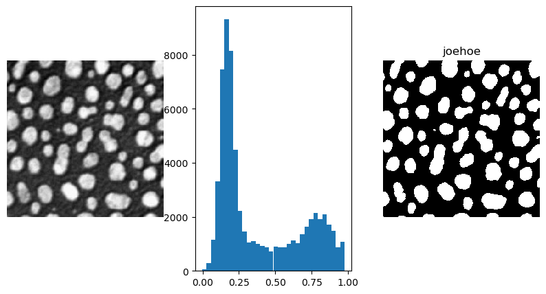
Fig. 3.9 Thresholding. On the left an image showing particles embedded in a substrate, the particles are brighter (whiter) than the background. This is also clearly visible in the histogram (center plot). On the right the thresholded image is shown. The threshold value is manually selected at \(t=0.5\).

There are many algorithms known that automatically calculate a suitable threshold for an image. In this section we will only look at one of them.

Isodata Thresholding

Isodata thresholding is a way to automatically find a threshold for a given gray value image \(f\). Consider a threshold \(t\) somewhere in the range of gray values in the image. Then we consider the mean of all pixels in the image with a gray value less then or equal to \(t\), call it \(m_L\) and the mean of all pixels with gray value greater than \(t\), let’s call that \(m_H\).

Isodate thresholding then finds a threshold such that

\[t = \frac{m_L+m_H}{2}\]

i.e. the value of \(t\) is such that \(t\) is halfway inbetween \(m_L\) and \(m_H\). Please not that both \(m_L\) and \(m_H\) are functions of \(t\). Therefor the above equation can be written as

\[t = \frac{m_L(t)+m_H(t)}{2} = m(t)\]

defining the function \(m\). A point \(t\) such that \(t=m(t)\) is called a fixed point of the function \(m\). Starting from an initial estimate \(t_0\) the fixed point can be found with fixed point iteration:

\[t_{i+1} = m(t_i)\]

In python this would result in the following code:

f = plt.imread(ipcv_image_path('cermet.png'))
t = 0.2
epst = 0.001
while 1:
    mL = f[f<=t].mean()
    mH = f[f>t].mean()
    t_new = (mL+mH)/2
    if abs(t-t_new) < epst:
        break
    t = t_new
    print(t)

0.3491027355194092
0.45121729373931885
0.480459988117218
0.48723137378692627
0.4890110492706299

The threshold value that is calculated is \(t=0.489\) and close to what we had manually selected.

In an exercise you are asked to implement the isodata thresholding algorithm using the histogram data instead of accessing all pixels in the entire image in every iteration.

3.2.3.1. Exercises

1. The isodata threshold algorithm was implemented in a previous section using the image directly. This obviously is overkill. We don’t need all individual pixel values, all we need is the histogram of the image.

   1. Given a histogram h of the image. The mid points of the bins are in array m. Give the expressions to calculate \(m_L\) and \(m_H\) as used in the isodata algorithm.

   2. Implement the isodata threshold algorithm using the histogram and not the individual pixel values (once the histogram is calculated of course). Note that epst should be related to the bin width of the histogram.

2. It is not that hard to prove that the isodata threshold algorithm really is 2-means clustering in disguise.

   1. Can you prove that?

   2. Using k-means clustering we can try to find more than just a background and object cluster.

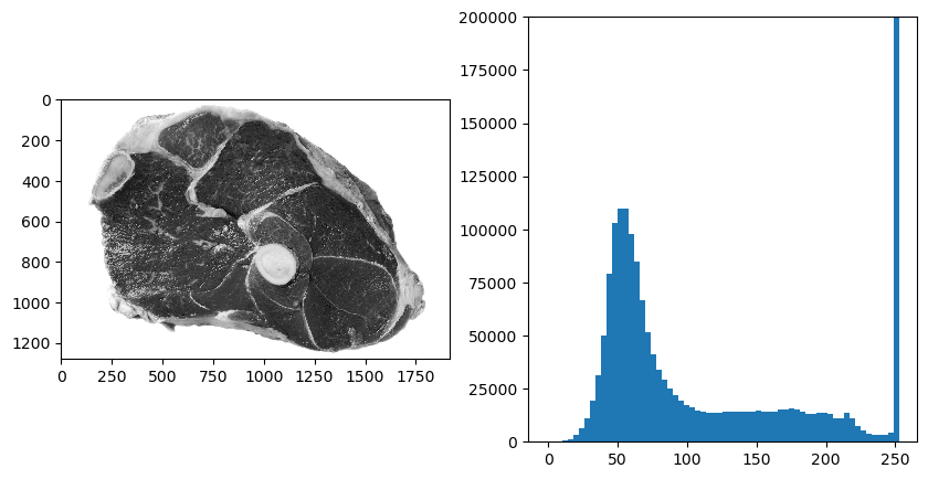
      Consider the image below of a piece of meat where we can distinguish a white background, a light gray fat area and dark gray for the muscle fiber.

      Show code for figure

      from ipcv.utils.files import ipcv_image_path
      
      f = plt.imread(ipcv_image_path('meat2.jpg'))[:,:,1];
      plt.subplot(121); plt.imshow(f);
      h, be = np.histogram(f, bins=64);
      plt.subplot(122);
      plt.bar(be[:-1], h, width=be[1]-be[0]);
      plt.ylim([0,200000])
      

      

      Using the sklearn.clustering.KMeans clustering algorithm it takes about 5 lines of python code to perform the segmentation into 3 clusters. The clustering/segmentation is certainly not perfect. Looking at the histogram and remembering what you learned about k-means clustering it should be clear why this segmantation will not perform perfectly. A Gaussian mixture model probably performs better.

      Your task to do the 3-means clustering and make an image where every pixel has value 0,1 or 2 according to the cluster it was assigned to. When displaying a label image a colorful colormap for imshow should be chosen (like the colormap jet).

   3. Formulating thresholding as k-means clustering also opens the possibility to ‘threshold’ color images directly without first looking at just the luminance values.

      Do 3-means clustering directly on the color image and again construct the label image. Compare the result with the label image obtained by 3-means classification of the gray value image.