5.2. Linear Operators: Convolutions
5.2.1. Linearity Definition
A linear operator is an operator that distributes over multiplicative weighted sums:
Let \(f\) and \(g\) be images and let \(a\) and \(b\) be scalars then \(\op L\) is a linear operator in case:
It is easy to prove that if the above holds, we can do the same for \(3,4,5,...\), any countable set of images (in fact linearity even requires you can do it for any set of images where summation becomes integration over a family of images).
5.2.2. Translation Invariance
The translation operator \(\op T_{\v t}\) translates an image over vector \(\v t\):
The translation over vector \(\v x\) is defined by
An operator \(\op O\) is called translation (or shift) invariant in case translation commutes with the operator:
An operator \(\op O\) is called translation invariant in case for all images \(f\)
or equivalently:
Translation invariance is an important assumption of the operators that we discuss in this section. However it is only strictly true in case the image domain is infinitely large (the entire \(\setR^2\) or \(\setZ^2\)). In practice image domains are bounded (an image has finite size) and thus translation invariance only approximately holds.
As is quite common in the image processing literature, in our theoretical analysis we assume infinite domains and translation invariant operators and we will deal with bounded domain in an adhoc fashion. The deviation from translation invariance is only noticible in a small region around the border (of width proportional to the maximal translation distance involved).
5.2.3. Linearity + Translation Invariance \(\Rightarrow\) Convolutions
Combining linearity with translation invariance leads to a unique characterization of linear, translation invariant operators: the convolutions. We first prove this result and then we will look at what type of image processing operator a convolution is. When first reading these notes you may want to start with a more intuitive explanation of the convolution operator and only after that return to this section.
A linear translation invariant operator \(\op L\) working on image \(f\) can be written as a convolution of \(F\) with the impulse response of \(\op L\). For a discrete operator:
where \(W = \op L \Delta\) is the impulse response function and \(\Delta\) is the discrete pulse:
Any function \(F\) can be written as a weighted linear combination of pulse functions:
As an example look at a very small \(2\times2\) image
Remember that these arrays are not matrices from linear algebra but small \(2\times2\) discrete images.
Note that \(\Delta(\v k - \v l) = \op T_{\v l} \Delta(\v i)\) and thus
or in function notation:
Applying the linear TI operator on both sides we get:
Using the fact that \(\op L\) is a linear operator we get:
and using the translation invariance of \(\op L\) we get
Evidently \(\op L\Delta\) is the impulse response of operator \(\op L\) and we write that as \(W=\op L\Delta\). So:
Adding the argument \(\v k\) again:
It is this last summation to get a new function \(\op L F\) out of a function \(F\) that we call the convolution of \(F\) with the impulse response \(W\):
5.2.4. Convolutions and Correlations
In the previous section we have defined the convolution of discrete function \(F\) with weight function or kernel \(W\) as:
in order to make the convolution easier to interpret we introduce the mirrored function \(W\mirror\):
Let \(W\) be a discrete function then we define the mirrored function \(W\mirror\) as:
As an example:
Common multiplicative factors are taken out of the braces and we write:
Note the in principle the \(W\) function is defined on the entire \(\setZ\). We only draw the values that are different from zero. Furthermore by convention we underline the origin.
Using the mirrored function we can write:
Based on this formula we can write down the following recipe for the convolution:
To calculate the convolution \(F\star W\):
Mirror \(W\) to get \(W\mirror\)
For all \(\v k\) do:
Shift \(W\mirror\) such that it’s origin is at position \(\v k\)
Multiply \(F(\v k + \v l)\) with \(W\mirror(\v l)\) for all \(\v l\).
Sum all values \(F(\v k + \v l)W\mirror(\v l)\)
Set the resulting value equal to the sum: \((F\star W)(\v k) = \sum_{\v l} F(\v k + \v l)W\mirror(\v l)\)
The operation where the kernel is not mirrored is called a correlation:
We have seen that it is the correlation operator that is easily interpreted and doesn’t require the mirroring of the kernel to start with. Indeed it is the simplest of the two operations and probably for that reason when researchers in Machinle (Deep) Learning talk about Convolutional Neural Networks they really talk about Correlational Neural Networks. In the next section where we look at properties of the convolution operator we will see that the convolution has some very nice mathematical properties that make the convolution the operator of choice in our context.
Let’s consider a simple example. A small discrete image is given as:
Show code
1import numpy as np
2
3rng = np.random.default_rng(seed=73482)
4F = rng.integers(0, 10, size=(12,12))
5print("F = ")
6print(F)
F =
[[6 5 3 2 4 6 7 2 0 7 8 1]
 [0 3 7 3 1 4 9 8 6 2 2 5]
 [3 0 7 6 5 3 7 9 9 1 8 5]
 [7 1 4 3 0 0 4 7 5 4 3 5]
 [3 2 5 0 9 3 7 0 8 5 3 1]
 [2 8 4 7 3 6 6 9 2 3 3 7]
 [6 4 2 2 8 6 9 6 0 9 5 3]
 [6 1 4 2 4 6 8 8 3 4 3 9]
 [6 0 3 3 7 5 3 2 3 2 5 6]
 [2 7 6 7 7 6 0 9 5 7 3 0]
 [4 0 2 8 1 0 4 8 2 4 6 3]
 [8 9 9 8 5 5 1 1 1 2 6 5]]
The convolution kernel and its mirror:
Show code
1W = 1/9 * np.array([[0, 0, 1, 0, 0],
2                    [0, 1, 1, 1, 0],
3                    [1, 1, 1, 1, 1]])
4print("9 W = ")
5print(9 * W)
6Wm = W[::-1, ::-1]
7print("9 Wm = ")
8print(9 * Wm)
9 W =
[[0. 0. 1. 0. 0.]
 [0. 1. 1. 1. 0.]
 [1. 1. 1. 1. 1.]]
9 Wm =
[[1. 1. 1. 1. 1.]
 [0. 1. 1. 1. 0.]
 [0. 0. 1. 0. 0.]]
The convolution of \(F\) and \(W\) is then given by
Show code
1from scipy.ndimage import convolve
2G = convolve(F,W)
3print("F * W = ")
4print(G)
F * W =
[[4 4 4 3 3 4 4 4 4 3 3 4]
 [3 3 4 4 3 4 5 6 5 3 3 4]
 [2 2 3 4 4 4 5 6 5 5 4 4]
 [3 3 3 3 4 4 5 4 6 5 4 4]
 [3 4 2 3 2 4 3 4 4 4 3 3]
 [3 3 4 3 5 4 6 5 4 3 4 3]
 [5 3 4 4 5 6 6 5 4 4 4 4]
 [4 3 3 3 5 6 5 5 5 3 4 5]
 [3 3 3 4 5 5 4 5 4 4 4 5]
 [3 3 4 5 4 3 4 4 4 4 4 3]
 [4 4 5 5 4 4 4 4 4 4 3 3]
 [4 5 5 4 4 4 2 2 3 3 4 4]]
It is important to select an appropriate convolution function. The one
in scipy.ndimage can work with multi dimensional images and allows
for many choices to deal with the border problem. Centered at the
point on the 4th row, 5th column we see the values
The mean of these values (rounded to an integer) is 4 as is given in the convolution result.
Evidently in case we are calculating the convolution sum for a point
near the border of the image the kernel may not fit entirely in the
image and we have to deal with the border problem. Please read the
documentation of the scipy.ndimage.convolve function what options
there are and what their effect is.
5.2.5. Convolutions in the Continuous Domain
Thus far we have considered only discrete image functions such that the convolution is a summation. Mathematical analysis of image processing often requires us to consider images defined on a continuous domain. For image functions \(f(\v x)\) where \(\v x\in\setR^d\) the convolution can also be defined, this time as an integral. Most of the theoretical properties are equally valid for continuous domain functions (images) as well.
5.2.5.1. The Convolutions Integral
Instead of a convolution sum in the discrete case we get a convolution integral in the continuous case. Again this follows from the assumption of a linear translation invariant operator. In the discrete domain we proved this by first writing the discrete image \(F\) as a summation of translated or shifted pulses \(\Delta(\v k - \v l)\).
In the continuous domain we need pulses translated to any position \(\v y\). The pulse should be different from zero in all locations except for the origin in such a way that:
It is this equation that defines the pulse function. We can only define this function as a limit. For an exanple see Fig. 5.4.
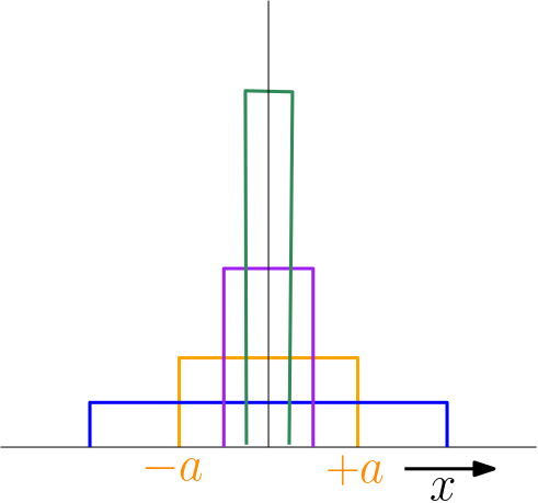
Fig. 5.4 Pulse as limit of block function. For \(a\rightarrow0\) the function value at \(x=0\) becomes infinitely large while keeping the area under the curve equal to one.
With this definition of the pulse function in the continuous domain we can prove:
A linear translation invariant operator \(\op L\) working on image \(f\) can be written as a convolution of \(f\) with the impulse response of \(\op L\).
where \(w\) is the impulse response \(w = L\delta\).
5.2.5.2. Convolutions and Differentiation
Differentiating image functions will be central in the next chapter where we look at the local structure of images. Remember that differentiation calculates the change in function value when the argument changes infinitesimally. Evidently infinitesimally small changes are not possible when dealing with discrete images only defined in its sample points. We can only approximate derivatives when working with discrete images (and we will do so in the next chapter).
In this subsection we therefore only consider images defined on a continuous domain. We will restrict ourselves to 2D images. For example consider the first order partial derivatives with respect to \(x\) and \(y\) of a convolution \((f\ast w)(x,y)\):
We will often write \(\partial_x\) as a shorthand of the partial derivative with respect to \(x\). Higher order derivatives are then denoted as \(\partial_{xx}\), \(\partial_{xxy}\) for the second order derivative with respect to \(x\) and the mixed order derivative where we take the second order derivative with respect to \(x\) combined with the first order derivative with respect to \(y\).
Let \(\partial_{\ldots}\) denote any partial derivative (of arbitrary order). Any derivative \(\partial_{\ldots}\) is a linear operator.
Based on the linearity of any derivative operator we have the following important theorem:
For any derivative \(\partial_{\ldots}\) and convolution \(f\ast w\) we have:
The importance of this theorem is twofold. Firstly regardless of whether the function \(f\) is differentiable or not, if we convolve with a kernel \(w\) that is differentiable, the convolution \(f\ast w\) is differentiable as well.
Secondly in case we only have a sampled (discrete) version \(F\) of the image (function) \(f\) we can discretize (sample) the derivative of the kernel function \(w\) and in that way approximage the derivative of the convolution. This will be central in our discussion of local structure in the next chapter.
5.2.5.3. From Convolution Integrals to Convolution Sums
Let \(F\) be the sampled version of some image function \(f\), i.e. \(F=\op S_B f\). We would like to calculate a sampled version of \(f\ast w\). Only in case the function \(f\) was perfectly bandlimited we can reconstruct \(f\) from its samples \(F\) by (sinc) interpolation. In most cases we can only reconstruct \(f\) approximately using interpolation:
where \(\op I_B\) is some linear interpolator characterized with interpolating function \(\phi\) with respect to the sampling grid generated by the column vectors in \(B\). The convolution of \(\hat f\) and a kernel \(w\) equals:
The approximation \(\hat f\) is build as a weighted summation of translated versions of the ‘interpolated kernel’ \(\phi\ast w\). Note that we can calculate \(\hat f\) at any location \(\v x\) in the continuous domain. In case we sample \(g = \hat f \ast w\) using the same grid, i.e. in the points \(B\v i\) we get:
Writing \(w_\phi\) for \(\phi\ast w\) and \(W_\phi[\v i]=w_\phi(B\v i)\):
Knowing that \(G\) is a aproximation of the sampling of \(f \ast w\) we may write:
Most of the image processing textbooks just state that a convolution integral in the continuous domain corresponds with a convolution sum in the discrete domain and that we just have to sample both the image and the kernel. This indeed is true in case \(\op S_B(w)=\op S_B(\phi\ast w)\) which is true in many important situations in practice.
Looking at the problem from a signal processing point of view we assume our image \(f\) to be bandlimited (or at least pre filtered to make it bandlimited before sampling). The corresponding ideal interpolation kernel is the sinc kernel (a perfect low pass filter). Then if \(w\) is bandlimited as well, we have \(w=w\ast\phi\) and in this case we have that \(\op S_B\left( f \ast w \right) = \op S_B f \star \op S_B w\). Note that your kernel should be bandlimited as well.
5.2.6. Properties of the Convolution Operator
Most if not all properties given in this subsection rely on the definition of both the image and the kernel (remember that in theory they play an equivalent role) on the infinite domain (either \(setZ^d\) or \(\setR^d\)). For bounded images these properties are not necessarily true although the errors are made in a small border region of the image.
5.2.6.1. The Impulse Response
If we convolve the pulse \(\Delta\) with a kernel \(W\) (and pulse \(\delta\) and kernel \(w\) in the continuous domain) we get
5.2.6.2. Commutativity
From a theoretical point of view when considering the convolution \(F\star W\) there is no special role for neither \(F\) nor \(G\). This is true in the continuous domain. In fact the convolution is a commutative operator:
The proof is left as an exercise for the reader.
5.2.6.3. Associativity
Again we leave the proof to the reader (and possibly for the exam…). The associativity of the convolution is a very important property in practice. By cascading convolutions with small kernels we obtain a convolution with a larger kernel. For instance:
Note that although in this way we can ‘make’ larger kernels, it still remains a linear translation invariant operator (i.e. a convolution). This is recognized in Convolutional Neural Networks where a lot of convolutions are cascaded but between two convolutions a non linear activation function is inserted. We will return to CNN’s in a later chapter.
5.2.6.4. Separable Convolutions
Consider a convolution:
This convolution can be dimensionally decomposed as:
We leave it as an exercise to prove that the above is true. Evidently the proof has nothing to do with the image \(F\) but only depends on the kernels being used. So the running average filter in a \(5\times5\) neighborhood can be implemented by first calculating the running average in a \(5\times1\) neighborhood, followed by a running average filter using a \(1\times5\) neighborhood.
The first 1D convolution runs along all the columns of the image whereas the second convolution runs along all rows. Note that for the 2D kernel we need to add 25 numbers whereas using the decomposition we need to add 5+5=10 numbers. In general we have the following result.
A function \(W(k,l)\) is called dimensional decomposable in case there are two 1D functions \(V(k)\) and \(H(l)\) such that
Note that we have used the numpy convention that the first axis of an array is the vertical axis and second axis is the horizontal axis. Given a decomposable kernel function \(W\) we can decompose the convolution:
In general for a 2D kernel with \(N\times N\) values requires \(N^2\) multiplications and additions whereas its decomposed form requires \(2N\) multiplications and additions. We will use this for the Gaussian convolution (discussed in a later subsection).
5.2.7. Often Used Convolutions
A lot of convolution kernels \(W\) used in practice are nowadays learned from data. We refer to the chapter for CNN’s for a short introduction.
In this section we look at only two convolutions: the uniform convolution and the Gaussian (derivative) convolution.
5.2.7.1. Uniform Convolutions
The uniform filter calculates a running average in a \((2M+1)\times(2N+1)\) window:
A uniform convolution is separable as discussed before. For instance for \(M=N=2\):
This lowers the computational complexity (assuming \(M\approx N\)) from \(\bigO(M^2)\) to \(\bigO(M)\). The computational complexity can be further reduced to \(\bigO(1)\). This will be dealt with in one of the exercises.
Show code for figure
 1import numpy as np
 2import matplotlib.pyplot as plt
 3from scipy.ndimage import uniform_filter
 4
 5f = plt.imread('source/images/cameraman.png')
 6plt.subplot(131)
 7plt.imshow(f, cmap='gray')
 8plt.axis('off')
 9
10g = uniform_filter(f, size=(11, 11))
11plt.subplot(132)
12plt.imshow(g, cmap='gray')
13plt.axis('off')
14
15plt.subplot(133)
16x = 90; y = 20; w = h = 100
17plt.imshow(g[y:y+h, x:x+w], cmap='gray')
18plt.axis('off')
19
20
21plt.savefig('source/images/uniform_cameraman.png')
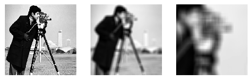
Fig. 5.5 Uniform Filter. Observe that in the smoothed image axis aligned artifacts are visible. The shape of the square kernel shows in the results.
5.2.7.2. Gaussian Convolutions
The Gaussian convolution uses a kernel:
Note that the Gaussian function is everywhere larger than zero, meaning that in principle the convolution kernel is infinitely large. In practice however we may truncate the kernel spatially due to the fact that the exponential function \(e^{-x^2}\) approaches zero for large \(x\).
The Gaussian (derivative) convolution will be discussed in more detail in a subsequent chapter.
Show code for figure
 1import numpy as np
 2import matplotlib.pyplot as plt
 3from scipy.ndimage import gaussian_filter
 4
 5f = plt.imread('source/images/cameraman.png')
 6plt.subplot(131)
 7plt.imshow(f, cmap='gray')
 8plt.axis('off')
 9
10g = gaussian_filter(f, sigma=(4, 4))
11plt.subplot(132)
12plt.imshow(g, cmap='gray')
13plt.axis('off')
14
15plt.subplot(133)
16x = 90; y = 20; w = h = 100
17plt.imshow(g[y:y+h, x:x+w], cmap='gray')
18plt.axis('off')
19
20
21plt.savefig('source/images/gaussian_cameraman.png')
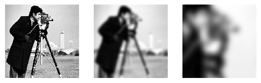
Fig. 5.6 Gaussian Filter. Observe that the smoothed result doesn’t show axis aligned artifacts that were visisble in the uniform filter.
The Gaussian (derivative) convolution will be discussed in the next chapter (and in one of the LabExerices).
Show code for figure
 1import numpy as np
 2import matplotlib.pyplot as plt
 3from scipy.ndimage import gaussian_filter
 4
 5f = plt.imread('source/images/cameraman.png')
 6plt.subplot(131)
 7plt.imshow(f, cmap='gray')
 8plt.axis('off')
 9
10g = gaussian_filter(f, sigma=(4, 4), order=(0,1))
11plt.subplot(132)
12plt.imshow(g, cmap='gray')
13plt.axis('off')
14
15h = gaussian_filter(f, sigma=(4, 4), order=(1,0))
16plt.subplot(133)
17plt.imshow(h, cmap='gray')
18plt.axis('off')
19
20
21plt.savefig('source/images/gaussian_derivatives_cameraman.png')
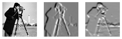
Fig. 5.7 Gaussian Derivative Filters. From left to right the original image \(F\), the first order derivative with respect to \(x\) (horizontal) and the first order derivative in the \(y\) direction.
5.2.8. Exercises
Linear Operator. From the definition of a linear image operator it follows that the zero image is mapped onto itself. This is often called the ‘origin’ or the (geometric( null vector. Can you prove this?
Translations and Translation Invariance.
Show that the convolution of function \(F\) with the shifted pulse \(\op T_{\v y}\Delta\) shifts (translates) the image \(F\): \((F\star \op T_{\v y}\Delta)(x) = F(\v x - \v y)\).
From the above we have that (in theory):
\[(F\star\op T_{\v y}\Delta)\star T_{-\v y}\Delta = F\]Show (with an example calculated using Python for example) that the above is not valid in practice.
Convolution versus Correlation.
The convolution is commutative, i.e. \(f\ast g = g\ast f\). This is not true for the correlation. Give the expression for \(f\ast_C g\) where \(g\) is on the left of the \(\ast_C\) and \(f\) on the right.
The convolution is associative, i.e. \((f\ast g)\ast h=f\ast(g\ast h)\). That is not true for the correlation \(\ast_C\). Give the expression for \((f\ast_C g)\ast_C g\).
Commutative Convolution. Prove that the (discrete) convolution is commutative.
Associative Convolution. Prove that the (discrete) convolution is associative.