6.2. Local Structure

In the introduction to this chapter we have shown for 1D function \(f\) that knowing the derivatives of \(f\ast G^s\) allows us to approximate the smoothed function using its truncated Taylor series. For a 1D function we cam approximate \(f^s=f^0\ast G^s\) in 2nd order as

\[f^s(a+x) = f^s(a) + x f^s_x(a) + \tfrac{1}{2} x^2 f^s_{xx}(a)\]

where we also observed that the approximation holds true in the neighborhood \(x\in[-\alpha s,+\alpha s]\) (with \(\alpha\) somewhere in the region from one to two), see Fig. 6.9. The collection of derivatives in a point \(a\) up to order \(N\) are often called the N-jet 1.

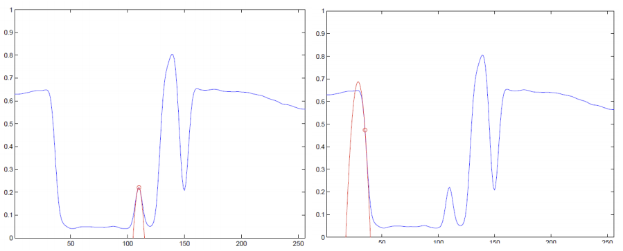
Fig. 6.16 Types of 1D neighborhoods in 2-jet. On the left at point \(a\) the first order derivative is almost zero and the function locally looks like a parabola. On the right the first order derivative dominates and the function locally looks like a straight line.

For 1D 2-jet a function \(f^s(a+x)\) around point \(a\) is easily characterized given the derivatives \(f^s_x\) and \(f^s_{xx}\). If the first order derivative dominates (i.e. is large in absolute value) the function locally looks like a linear function with a strong (positive or negative) slope. In case the first order derivative is small the neighborhood is dominated by the second order derivative \(f^s_{xx}\). The function locally locally looks like an upward pointing or downward pointing parabola. This is illustrated in Fig. 6.16.

The local Taylor approximation can be easily extended to two dimensional functions (images):

Definition 6.7 (Taylor Approximation for Images)

Let \(f^s = f^0 \ast G^s\) then we may approximate the neighborhood of point \(\v a\) with the second order Taylow polynomial:

\[\begin{split}f^s(\v a + \v x) \approx f^s(\v a) + \v x\T \begin{pmatrix}f^s_x(\v a)\\f^s_y(\v a)\end{pmatrix} + \tfrac{1}{2} \v x\T \begin{pmatrix} f^s_{xx}(\v a) & f^s_{xy}(\v a)\\ f^s_{xy}(\v a) & f^s_{yy}(\v a) \end{pmatrix} \v x\end{split}\]

where:

\[\begin{split}\nabla f^s = \begin{pmatrix}f^s_x(\v a)\\f^s_y(\v a)\end{pmatrix}\end{split}\]

is the gradient vector and

\[\begin{split}H_{f^s}(\v a) = \begin{pmatrix} f^s_{xx}(\v a) & f^s_{xy}(\v a)\\ f^s_{xy}(\v a) & f^s_{yy}(\v a) \end{pmatrix}\end{split}\]

is the Hessian matrix. Thus

\[f^s(\v a + \v x) \approx f^s(\v a) + \v x\T \nabla f^s(\v a) + \tfrac{1}{2} \v x\T H_{f^s}(\v a) \v x\]

In this chapter we assume throughout that the (most often fixed) scale \(s\) is known a priori. That is why we will often omit the scale \(s\) (for brevity) from the formulas and write:

\[f(\v a + \v x) \approx f(\v a) + \v x\T \nabla f(\v a) + \tfrac{1}{2} \v x\T H_{f}(\v a) \v x\]

but carefully note that we will always assume a fixed scale \(s>0\).

Show code for figure

import numpy as np
import matplotlib.pyplot as plt

plt.close('all')

N = 15
x = np.arange(-N, N+1)
X, Y = np.meshgrid(x, x)

e1 = np.array([1,0])
def rotate(v, phi):
    R = np.array([[np.cos(phi), -np.sin(phi)],
                  [np.sin(phi), np.cos(phi)]])
    return R @ v


fig = plt.figure(figsize=(5,8))
plt.tight_layout()

iphis = [(1, 0), (3, np.pi/4), (5, np.pi/2)]
for i, phi in iphis:
    (fx, fy) = 5* rotate(e1, phi)
    F = fx * X + fy * Y + 128

    
    ax2d = fig.add_subplot(len(iphis), 2, i)
    ax2d.imshow(F, vmin=0, vmax=255, cmap = plt.cm.gray)
    ax2d.contour(F)
    ax2d.set_xlabel('x')
    ax2d.set_ylabel('y')
    ax2d.xaxis.set_ticks([])
    ax2d.yaxis.set_ticks([])
    ax2d.arrow(15, 15, 2*fx, 2*fy, length_includes_head=True, width=0.5, head_width=2);


    ax3d = fig.add_subplot(len(iphis), 2, i+1, projection='3d')
    surf = ax3d.plot_surface(X, Y, F, rstride=1, cstride=1, linewidth=1,
                             antialiased=False)
    ax3d.set_xlabel('x')
    ax3d.set_ylabel('y')
    ax3d.xaxis.set_ticks([])
    ax3d.yaxis.set_ticks([])
    ax3d.zaxis.set_ticks([])
plt.savefig('source/images/2d_nbhs.png')

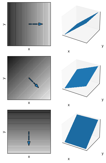
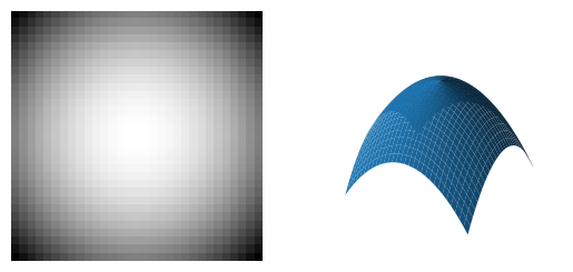
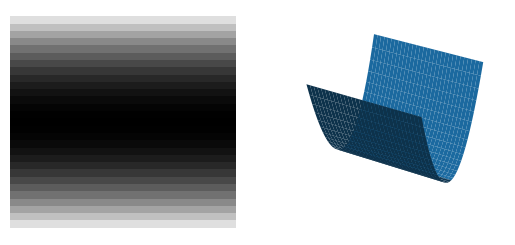
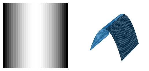
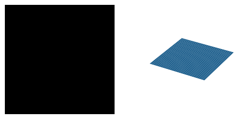
Fig. 6.17 Typical Neighborhoods for vanishing Hessian matrix. In the left column an image rendering of a first order Taylor polynomial for 3 different gradient vectors. The gradient vectors are shown drawn on top of the image. Also shown are a few isophotes (lines of equal gray value). Note that the \(y\) axis points downwards. In the second colomn the same neighborhoods are shown rendered as function surface.

This definition shows that the image locally around point \(\v a\) can be approximated with a multivariate polynomial in which the coefficients are proportional to the partial derivatives of the image function \(f^s\). Also for this Taylor approximation the region in which the approximation holds within reasonable accuracy is in the order of a distance \(s\) to \(2s\) from point \(a\).

For a 2D function the geometrical interpretation of the function surface given its derivatives is a bit more difficult than it is for 1D functions.

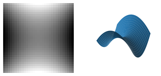
First we consider the case where the gradient vector dominates the Hessian matrix. In the extreme case we consider all second order derivatives equal zero (see Fig. 6.17).

Observe that the neighborhoods are basically the same except for a different orientation as given by the direction of the gradient vector. In the next subsection we will introducte the gradient gauge coordinate system where one of the basis vectors is pointing in the gradient direction. Note that in every point in the image we have a possibly different gradient coordinate system to describe the local neighborhood.

6.2.1. Gradient Gauge Coordinate System

In the gradient gauge coordinate system we attach a coordinate frame, with basis vectors \(\v e_v\) and \(\v e_w\), to the data at every point by setting the \(\v e_w\) in the direction of the gradient vector:

\[\begin{split}\v e_w = \frac{\nabla f(\v x)}{\|\nabla f(\v x)\|} = \frac{1}{\sqrt{(f_x(\v x))^2 + (f_y(\v x))^2}} \begin{pmatrix}f_x(\v x) \\ f_y(\v x)\end{pmatrix}\end{split}\]

where each \(f\) term should be read as \(f^s\). Also for brevity we leave out the argument \(\v x\) often in case that is evident from the context.

(6.1)\[\begin{split}\v e_w = \frac{\nabla f}{\|\nabla f\|} = \frac{1}{\sqrt{(f_x)^2 + (f_y)^2}} \begin{pmatrix}f_x \\ f_y\end{pmatrix}\end{split}\]

The \(\v e_v\) is perpendicular to \(\v e_w\):

(6.2)\[\begin{split}\v e_v = \frac{1}{\sqrt{(f_x)^2 + (f_y)^2}} \begin{pmatrix}f_y \\ -f_x\end{pmatrix}\end{split}\]

Show code for figure

from matplotlib.pylab import *
from scipy.ndimage import gaussian_filter

def gD(f, scales, orders):
    return gaussian_filter(f, scales, orders)

f0 = imread('source/images/cameraman.png')
fs = gD(f0,2,0)
fsy = gD(f0,2,(1,0))[::8,::8]
fsx = gD(f0,2,(0,1))[::8,::8]
gradnorm = hypot(fsx,fsy)
M,N = f0.shape[:2]
X,Y = meshgrid(arange(0,M,8),arange(0,N,8))
imshow(fs, cmap='gray')
quiver(X, Y, fsx, fsy, angles='xy', scale_units='xy', scale=0.01, color='r')
quiver(X, Y, -fsy, fsx, angles='xy', scale_units='xy', scale=0.01, color='b')
axis('off')

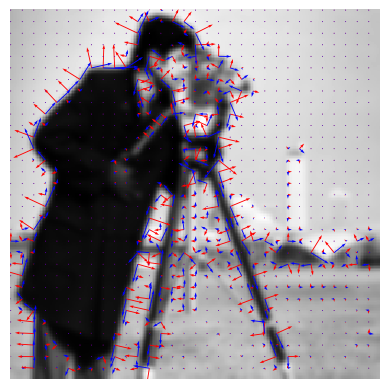
Fig. 6.18 Gradient Gauge Coordinate System. The red vectors (perpendicular to edges in the image) are in the \(\v e_w\) direction, the blue vectors are in the \(\v e_v\) direction.

The standard coordinate frame \((\v e_x, \v e_y)\) is a rather random one. If the photographer rotates his camera slightly the axes are rotated as well. Then the components of the gradient vector also change! But the direction and length of the gradient vector, as defined with respect to the image geometry, stays unaltered.

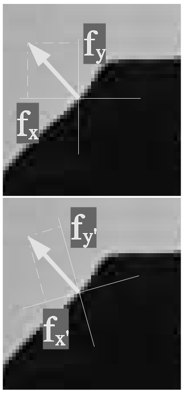
Fig. 6.19 Gradient vector. The gradient vector with respect to basis \((\v e_x, \v e_y)\) has different components \(f_x\) and \(f_y\) as the gradient vector measured in the \((\v e_{x'}, \v e_{y'})\) with components \(f_{x'}\) and \(f_{y'}\). Nevertheless the gradient vector points in the same direction with respect to the data geometry.

The gradient gauge is a coordinate system where the (local) coordinate system \((\v e_v, \v e_w)\) is fixed with respect to the image geometry.

Therefore we would like to express the image derivatives also with respect to these gauge coordinates. The derivative \(f_v\) is the derivative in the \(\v e_v\) direction, likewise \(f_w\) is the derivative in the \(\v e_w\) direction.

Evidently we can also express the image function \(f\) locally around the point \(\v a\) where we have calculated the derivatives as a Taylor polynomial but now with respect to the \((v, w)\) coordinates.

\[\begin{split}f(\v a + \v v) \approx f(\v a) + \v v\T \begin{pmatrix}f_v(\v a)\\f_w(\v a)\end{pmatrix} + \tfrac{1}{2} \v v\T \begin{pmatrix}f_{vv}(\v a) & f_{vw}(\v a)\\f_{vw}(\v a) & f_{ww}(\v a)\end{pmatrix} \v v\end{split}\]

where \(\v v = v \v e_v + w \v e_w\). The goal now is to express the derivatives in \(\v e_v\) and \(\v e_w\) directions in terms of the derivatives in the \(\v e_x\) and \(\v e_y\) direction. Because this is indeed possible we can calculate the derivatives in the gradient gauge by calculating the derivatives in the standard basis. These derivatives \(f_x\), \(f_y\), \(f_{xx}\) etc are aligned with the standard image axes and thus can be calculated for all points in an image with Gaussian derivative convolutions which can be efficiently computed with separable convolutions.

There are two ways we can calculate the derivatives with respect to the gradient gauge coordinates. The first one uses directional derivatives. Let \(\v e_r = (r_x\; r_y)\T\) be a direction vector then the derivative \(f_r\) is defined as:

\[\begin{split}f_r(\v a) &= \lim_{dr\rightarrow0} \frac{f(\v a + dr \;\v e_r)-f(\v a)}{dr}\\ &= \lim_{dr\rightarrow0} \frac{f(\v a) + dr \;\v e_r\T\nabla f(\v a) -f(\v a)}{dr}\\ &= \v e_r\T\nabla f(\v a) = r_x f_x(\v a) + r_y f_y(\v a)\end{split}\]

or again omitting the argument \(\v a\), the directional derivative in \(\v e_r\) direction is

(6.3)\[f_r = r_x f_x + r_y f_y\]

For the directional derivative \(f_v\) and \(f_w\) in the directions \(\v e_v\) and \(\v e_w\) respectively (see Eq. (6.1) and Eq. (6.2)) we have:

Theorem 6.8 (First Order Directional Derivatives in Gradient Gauge)

The first order directional derivatives in the gradient gauge coordinate system are:

\[\begin{split}f_v(\v a) &= 0\\ f_w(\v a) &= \sqrt{(f_x(\v a))^2 + (f_y(\v a))^2} = \|\nabla f(\v a)\|\end{split}\]

Proof

We only give the proof for the \(\v e_w\) direction and leave the proof for the \(\v e_v\) direction to the reader.

Consider the direction \(\v e_r = \v e_w\) where:

\[\begin{split}r_x &= \frac{f_x}{\sqrt{f_x^2+f_y^2}}\\ r_y &= \frac{f_y}{\sqrt{f_x^2+f_y^2}}\end{split}\]

Using Eq. (6.3) we have:

\[f_w = r_x f_x + r_y f_y = \frac{f_x}{\sqrt{f_x^2+f_y^2}} f_x + \frac{f_y}{\sqrt{f_x^2+f_y^2}} f_y = \sqrt{f_x^2+f_y^2}\]

The argument \(\v a\) in the above theorem (Proof 6.8) is given explicitly to stress the fact that the derivative \(f_v\) is not a constant function (zero). Only in the point where the derivative is calculated this is true. So the function seen from a point \(\v a\) is locally flat in the \(\v e_v\) direction.

For the second order derivatives we can use the same line of thought. For instance \(f_{ww}\) is the directional derivative in \(\v e_w\) direction of \(f_w\). For all three partial derivatives in the Hessian matrix we have:

Theorem 6.9 (Second Order Derivatives in the Gradient Gauge)

\[\begin{split}f_{vv} &= \frac{1}{f_x^2+f_y^2}\left( f_x^2 f_{yy} - 2f_x f_y f_{xy} + f_y^2 f_{xx} \right)\\ f_{vw} &= \frac{1}{f_x^2+f_y^2}\left( (f_y^2-f_x^2)f_{xy} + f_x f_y (f_{xx}-f_{yy}) \right)\\ f_{ww} &= \frac{1}{f_x^2+f_y^2}\left( f_x^2 f_{xx} + 2 f_x f_y f_{xy} + f_y^2 f_{yy} \right)\end{split}\]

Proof

We only give the proof for \(f_{ww}\) and leave the rest to the reader.

\[\begin{split}f_{ww} &= \pfrac{f_w}{w}\\ &= \pfrac{}{w} \sqrt{f_x^2 + f_y^2}\\ &= \frac{1}{2 \sqrt{f_x^2 + f_y^2}}\pfrac{}{w}\left(f_x^2+f_y^2\right)\\ &= \frac{1}{2 \sqrt{f_x^2 + f_y^2}}\left( 2 f_x \pfrac{f_x}{w} + 2 f_y\pfrac{f_y}{w}\right)\\ &= \frac{1}{\sqrt{f_x^2 + f_y^2}}\left( f_x \left[\frac{f_x}{\sqrt{f_x^2+f_y^2}}f_{xx} + \frac{f_y}{\sqrt{f_x^2+f_y^2}}f_{xy}\right] + f_y\left[ \frac{f_x}{\sqrt{f_x^2+f_y^2}} f_{xy} + \frac{f_y}{\sqrt{f_x^2+f_y^2}} f_{yy}\right]\right)\\ &= \frac{1}{f_x^2 + f_y^2}\left( f_x^2 f_{xx} + 2 f_x f_y f_{xy} + f_y^2 f_{yy} \right)\end{split}\]

The second way to calculate the directional derivatives in the gradient gauge coordinate system is more geometrical in nature. The coordinate axes \(\v e_v\) and \(\v e_w\) are rotated versions of the standard \(\v e_x\) and \(\v e_y\) basis vectors. Observe that

\[\begin{split}\begin{pmatrix}\v e_v & \v e_w\end{pmatrix} = \frac{1}{\sqrt{f_x^2+f_y^2}} \begin{pmatrix}f_y & f_x\\-f_x & f_y\end{pmatrix} \begin{pmatrix}\v e_x & \v e_y\end{pmatrix} = \frac{1}{\sqrt{f_x^2+f_y^2}} \begin{pmatrix}f_y & f_x\\-f_x & f_y\end{pmatrix} \begin{pmatrix}1&0\\0&1\end{pmatrix}\end{split}\]

The rotation matrix

\[\begin{split}R = \frac{1}{\sqrt{f_x^2+f_y^2}} \begin{pmatrix}f_y & f_x\\-f_x & f_y\end{pmatrix}\end{split}\]

thus rotates the standard basis vectors into the basis vectors in the gradient gauge coordinate system. Thus given a point with coordinates \(\v x = (x\;y)\T\) in the standard frame is represented with coordinates \(\v v = (v\;w)\T\) in the gradient coordinate system:

\[\v v = R\T \v x\]

So if we now look at the Taylor approximation:

\[f(\v a + \v x) = f(\v a) + \v x\T \nabla f(\v a) + \tfrac{1}{2}\v x\T H_f(\v a) \v x\]

we may substitute \(\v x = R\v v\):

\[f(\v a + R\v v) = f(\v a) + \v v\T R\T \nabla f(\v a) + \v v\T R\T H_f(\v a) R \v v\]

Thus the gradient vector with respect to the gradient coordinate system is:

\[\begin{split}\begin{pmatrix}f_v\\f_w\end{pmatrix} &= R\T \begin{pmatrix}f_x\\f_t\end{pmatrix}\\ &= \frac{1}{\sqrt{f_x^2+f_y^2}} \begin{pmatrix}f_y & -f_x\\f_x & f_y\end{pmatrix} \begin{pmatrix}f_x\\f_y\end{pmatrix}\\ &= \frac{1}{\sqrt{f_x^2+f_y^2}} \begin{pmatrix}f_x f_y - f_x f_y\\f_x^2+f_y^2\end{pmatrix}\\ &= \begin{pmatrix}0\\\sqrt{f_x^2+f_y^2}\end{pmatrix}\end{split}\]

This is the same as we found using the directional derivative operator. For the Hessian matrix we have:

\[\begin{split}\begin{pmatrix}f_{vv} & f_{vw}\\ f_{vw}& f_{ww}\end{pmatrix} = R\T \begin{pmatrix}f_{xx} & f_{xy}\\ f_{xy}& f_{yy}\end{pmatrix} R\end{split}\]

We leave it as an exercise to the reader to substitute the expression for \(R\) to show that the values for \(f_{vv}\), \(f_{vw}\) and \(f_{ww}\) are the same as calculated with the expression for a directional derivative.

6.2.1.1. Canny Edge Detector

Edges in 1D

In 1D an edge is simple to define. It’s the position (\(x\) value) of the transition from a low value to a high value of the signal (function) or the transition from high to low. In the figure below the canonical edges in a 1D signal are given. What characterizes a point on an edge is:

• its position (\(x\) value)

• the change in function (gray) value across the edge

The mathematical way to express change is by using derivatives. The derivative \(f'(x)\) is proportional to the change in the function value \(f\) when the value of \(x\) is increased slightly.

Consider the canonical edge profile, gradually changing from low to high values. The derivative is almost zero far to the left of the edge, then it gradually increases until it reaches a maximum value (where the edge is) and from there decreases gradually to zero again.

Show code for figure

from matplotlib.pylab import *
from scipy.special import erf

x = linspace(-5,5,100)
f = (erf(x)+1)/2
subplot(3,1,1)
plot(x,f,lw=3)
ylim(-0.1,1.1)
title(r'\$f\$')
axis('off')
subplot(3,1,2)
plot(x[:-1]+0.05, diff(f), lw=3)
ylim(ymin=-.1)
title(r"\$f'\$")
axis('off')
subplot(3,1,3)
plot(x[:-2]+0.1, diff(f,n=2), lw=3)
title(r"\$f''\$")
axis('off')
savefig("source/images/oneDedge.png")

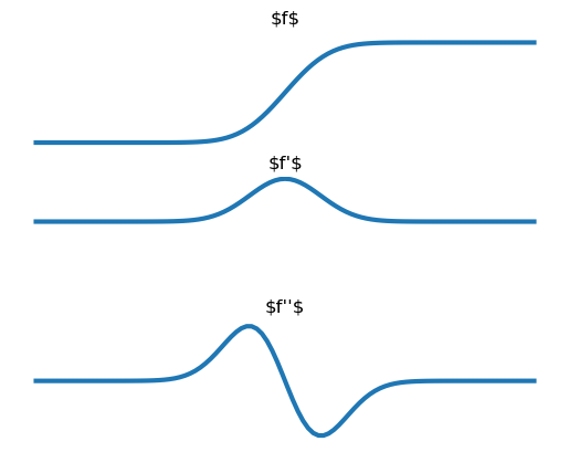
Fig. 6.20 One Dimensional Edge.

Thus an edge is characterized as a point where the first order derivative (in absolute sense) is large and the second order derivative is almost zero (the change of the first order derivative is minimal):

\[\begin{split}f'(x) \gg 0\\ f''(x) \approx 0\end{split}\]

When implementing such a scheme to work on sampled images we should be careful. The first condition is simple: \(f'(x)\gg 0\) is implemented as a comparison with some threshold \(t\): \(f'(x)>t\). The second condition is troublesome. For course sampled images the second order derivative could change from a relatively large positive value on the left of an edge to a relatively small negative value on the right. Then nowhere near the edge the second order derivative will be equal to zero. We therefore better find a way to check for such zero crossings. We leave that for a Lab Exercise.

Edges in 2D

An edge in 2D is most often an edge in 1D where the direction in which to look for the edge can and will differ from point to point in an image. Which direction to choose then? Imagine you are standing on a mountain with a very smooth surface. The height of the surface above sea level (say) can be expressed as a function \(h(x,y)\) (assuming of course that the flat earth assumption is—locally—reasonable). The assumed smoothnes of the function implies that the function can be differentiated.

Standing on that mountain we can turn around at the same spot. In one particular direction we find the mountain is increasing in height maximally. The slope in that direction is the maximal slope of the mountain at that particular point. In the perpendicular direction the slope is zero. That is the direction of the curve of equal height.

Mathematically the direction of maximal slope in a point \(\v a\) is given by the direction of the gradient vector \((\nabla f )(\v a)\):

\[\begin{split}(\nabla f)(\v a) = \matvec{c}{f_x(\v a)\\f_y(\v a)}\end{split}\]

the norm of the gradient vector is equal to the maximal slope.

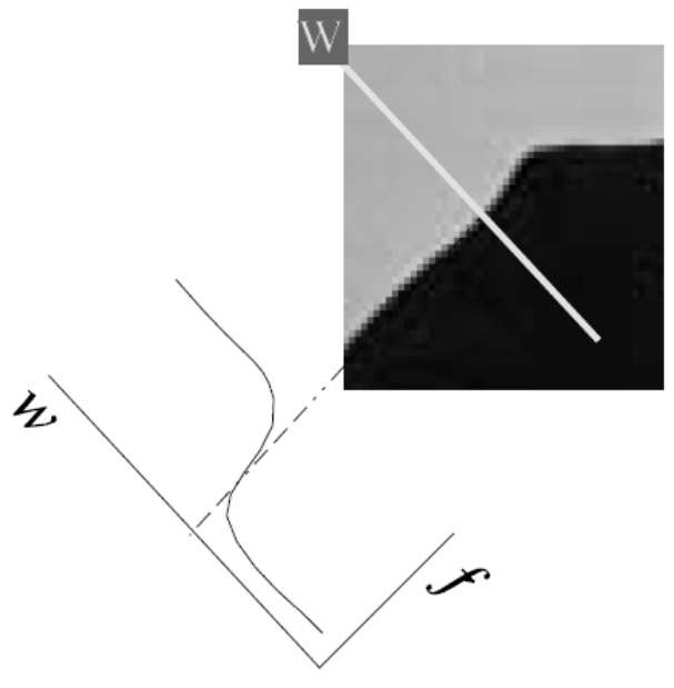
Fig. 6.21 Definition of Canny Edge.

When looking for edges it is evident to look in the gradient direction. The gradient direction by convention is called the \(w\)-direction and the unit vector in that direction is denoted as \(\v e_w\). The direction perpendicular to the gradient vector is called the \(v\)-direction with corresponding unit vector \(\v e_v\). The vectors \(\v e_v\) and \(\v e_w\) form a right handed orthonormal frame. Please note that at each point in the image we may have a different gradient frame.

In 2D we thus can characterize an edge point with derivatives in the \(\v e_w\) direction:

\[\begin{split}f_w(\v a) &\gg 0\\ f_{ww}(\v a) &\approx 0\end{split}\]

The derivatives in the \(v\) and \(w\) direction can be expressed in terms of the derivatives in \(x\) and \(y\) direction, leading to:

\[\begin{split}\sqrt{f_x^2(\v a)+f_y^2(\v a)} &\gg 0\\ \frac{f_x(\v a)^2f_{xx}(\v a) + 2 f_x(\v a) f_y(\v a) f_{xy}(\v a) + f_y^2(\v a) f_{yy}(\v a)}{f_x^2(\v a)+f_y^2(\v a)} &\approx0\end{split}\]

Because we are looking at edges, where by definition \(f_w>0\), the division in the second equation by \(f_w^2\) won’t lead to numerical problems. I.e. at the location of edges it won’t. But at a lot of areas in the image the gradient is very small (regions of constant gray value) and in such regions the second expression will lead to numerical problems. In practice therefore we most often use the conditions:

\[\begin{split}f_w(\v a) &\gg 0\\ f_w^2(\v a)f_{ww}(\v a) &\approx 0\end{split}\]

leading to the following conditions expressed in cartesian coordinates:

\[\begin{split}\sqrt{f_x^2(\v a)+f_y^2(\v a)} &\gg 0\\ f_x(\v a)^2f_{xx}(\v a) + 2 f_x(\v a) f_y(\v a) f_{xy}(\v a) + f_y^2(\v a) f_{yy}(\v a)&\approx0\end{split}\]

Calculating the left hand sides of both conditions are ‘one liners’ in Python/Numpy. Comparing the gradient norm with a threshold is also simple but again finding the sample points where the second order derivative in \(\v e_w\) direction is zero is troublesome. Instead of looking for small values of the second order derivative it is better to search for the zero crossings.

6.2.2. Curvature Gauge Coordinate System

The gradient gauge previously discussed before can only be used in case in a point \(\v a\) the gradient does not vanish. In case \(\nabla f(\v a)\approx \v 0\) the gradient gauge cannot be defined. In such cases the curvature gauge is often more usable. The Taylor approximation of local neigborhood in that case looks like:

\[f(\v a + \v x) = f(\v a) + \tfrac{1}{2} \v x\T H_f(\v a) \v x\]

Apart from the constant term we recognize that the function landscape is described as a quadratic form. From linear algebra class you know that we find a coordinate system in which the quadratic form matrix becomes a diagonal matrix.

The required coordinate system to diagonalize the quadratic form is formed by the two eigenvectors of the symmetric Hessian matrix (and because the the Hessian matrix is symmetric the eigenvectors are orthogonal). Let \(\v e_p\) and \(\v e_q\) be the two normalized eigenvectors and let \(R\) be the rotation matrix that takes the standard basis of vectors \(\v e_x\) and \(\v e_y\) into the basis of vectors \(\v e_p\) and \(\v e_q\).

The two eigenvalues of the Hessian matrix

\[\begin{split}H_f = \begin{pmatrix}f_{xx} & f_{xy}\\f_{xy} & f_{yy}\end{pmatrix}\end{split}\]

are

\[\begin{split}f_{pp} &= \half\left(f_{xx} + f_{yy} - \sqrt{(f_{xx}-f_{yy})^2 + 4 f_{xy}^2}\right)\\ f_{qq} &= \half\left(f_{xx} + f_{yy} + \sqrt{(f_{xx}-f_{yy})^2 + 4 f_{xy}^2}\right)\end{split}\]

and the eigenvectors are:

\[\begin{split}\v v_p &= \begin{pmatrix} f_{xx}-f_{yy} - \sqrt{(f_{xx}-f_{yy})^2 + 4 f_{xy}^2}\\2 f_{xy} \end{pmatrix}\\ \v v_q &= \begin{pmatrix} f_{xx}-f_{yy} + \sqrt{(f_{xx}-f_{yy})^2 + 4 f_{xy}^2}\\2 f_{xy} \end{pmatrix}\end{split}\]

and the basis vectors in the curvature gauge are:

\[\v e_p = \frac{\v v_p}{\|\v v_p\|}, \qquad \v e_q = \frac{\v v_q}{\|\v v_q\|}\]

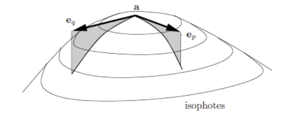
Fig. 6.22 Curvature Gauge. for a point \(\v a\) where \(\nabla f(\v a)\approx 0\). For this parabola shaped function with top pointing upwards we have \(f_{pp}\approx f_{qq}\ll0\).

Within the curvature gauge coordinate system, still assuming that \(\nabla f(\v a)\approx 0\), we have:

\[\begin{split}f(\v a + R\v p) \approx f(\v a) + \half \v p\T \pmatrix{f_{pp}&0\\0&f_{qq}} \v p\end{split}\]

where \(\v p = (p\; q)\T\) and \(R = (\v e_p\; \v e_q)\) is the rotation matrix that takes the vectors in the standard basis and produces the basis vectors in the curvature gauge coordinate system.

Show code for figures in table

import numpy as np
import matplotlib.pyplot as plt

plt.close('all')

N = 15
p = np.arange(-N, N+1)
P, Q = np.meshgrid(p, p)


# Dark Blob
f = 3 * P**2 + 3 * Q**2
figDBlob = plt.figure()
plt.subplot(1,2,1)
plt.imshow(f, cmap=plt.cm.gray)
plt.axis('off')
plt.subplot(1,2,2, projection='3d')
plt.gca().plot_surface(P, Q, f)
plt.axis('off')


# Bright Blob
f = -3 * P**2 - 3 * Q**2
figBBlob = plt.figure()
plt.subplot(1,2,1)
plt.imshow(f, cmap=plt.cm.gray)
plt.axis('off')
plt.subplot(1,2,2, projection='3d')
plt.gca().plot_surface(P, Q, f)
plt.axis('off')


# Dark Bar
f = 0 * P**2 + 3 * Q**2
figDBar = plt.figure()
plt.subplot(1,2,1)
plt.imshow(f, cmap=plt.cm.gray)
plt.axis('off')
plt.subplot(1,2,2, projection='3d')
plt.gca().plot_surface(P, Q, f)
plt.axis('off')



# Bright Bar
f = -3 * P**2 + 0 * Q**2
figBBar = plt.figure()
plt.subplot(1,2,1)
plt.imshow(f, cmap=plt.cm.gray)
plt.axis('off')
plt.subplot(1,2,2, projection='3d')
plt.gca().plot_surface(P, Q, f)
plt.axis('off')



# Flat
f = 0 * P**2 + 0 * Q**2
figFlat = plt.figure()
plt.subplot(1,2,1)
plt.imshow(f, cmap=plt.cm.gray)
plt.axis('off')
plt.subplot(1,2,2, projection='3d')
plt.gca().plot_surface(P, Q, f)
plt.axis('off')



# Saddle
f = -3 * P**2 + 3 * Q**2
figSaddle = plt.figure()
plt.subplot(1,2,1)
plt.imshow(f, cmap=plt.cm.gray)
plt.axis('off')
plt.subplot(1,2,2, projection='3d')
plt.gca().plot_surface(P, Q, f)
plt.axis('off')











figDBlob.savefig('source/images/curvatureDBlob.png')
figBBlob.savefig('source/images/curvatureBBlob.png')
figDBar.savefig('source/images/curvatureDBar.png')
figBBar.savefig('source/images/curvatureBBar.png')
figFlat.savefig('source/images/curvatureFlat.png')
figSaddle.savefig('source/images/curvatureSaddle.png')

Table 6.1 Curvature Gauge Taxonomy.

Name	Condition	Image / Surface
Dark Blob	\(f_{pp}\approx f_{qq} \gg 0\)
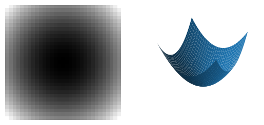
Bright Blob	\(f_{pp}\approx f_{qq} \ll 0\)
Dark Bar	\(f_{pp}\approx0, f_{qq}\gg 0\)
Bright Bar	\(f_{pp}\ll 0, f_{qq}\approx 0\)
Flat	\(f_{pp}\approx f_{qq}\approx 0\)
Saddle	\(f_{pp}\ll 0, f_{qq}\gg 0\)

6.2.2.1. Line Detector

Show code for figure

import numpy as np
import matplotlib.pyplot as plt

plt.close('all')

try:
    f = plt.imread('../../source/images/schema.png')
except:
    f = plt.imread('source/images/schema.png')

from scipy.ndimage import gaussian_filter as gD
s = 1
fs = gD(f, s)
fsx = gD(f, s, (0,1))
fsy = gD(f, s, (1,0))
fsxx = gD(f, s, (0,2))
fsxy = gD(f, s, (1,1))
fsyy = gD(f, s, (2,0))

plt.figure(figsize=(10, 10))
plt.subplot(221)
plt.imshow(f, cmap=plt.cm.gray)
ax = plt.gca()
plt.title('Original Image f')
ax.axes.xaxis.set_ticks([])
ax.axes.yaxis.set_ticks([])


plt.subplot(222, projection='3d')
x = 140
y = 195
w = h = 21
detail = fs[y:y+h, x:x+w]
xs = np.arange(21)
X, Y = np.meshgrid(xs, xs)
ax = plt.gca()
ax.plot_surface(X, Y, detail, cmap=plt.cm.gray)
plt.title('Surface plot of T-junction')
ax.axes.xaxis.set_ticks([])
ax.axes.yaxis.set_ticks([])



plt.subplot(223)
plt.imshow(-1.0 * (f<0.5), cmap=plt.cm.gray)
plt.title('Thresholded Image')
ax = plt.gca()
ax.axes.xaxis.set_ticks([])
ax.axes.yaxis.set_ticks([])



fw = np.hypot(fsx, fsy)
fpp = (fsxx + fsyy - np.sqrt((fsxx - fsyy)**2 + 4 * fsxy**2))/2
fqq = (fsxx + fsyy + np.sqrt((fsxx - fsyy)**2 + 4 * fsxy**2))/2

A = 1
B = 1
C = 1
lines = (1 - np.exp(-fqq**2/A)) * np.exp(-fpp**2/B) * np.exp(-fw**2/C)
plt.subplot(224)
plt.imshow(-lines, cmap=plt.cm.gray)
plt.title('Line Detection')
ax = plt.gca()
ax.axes.xaxis.set_ticks([])
ax.axes.yaxis.set_ticks([])
plt.savefig('source/images/linedetection.png')

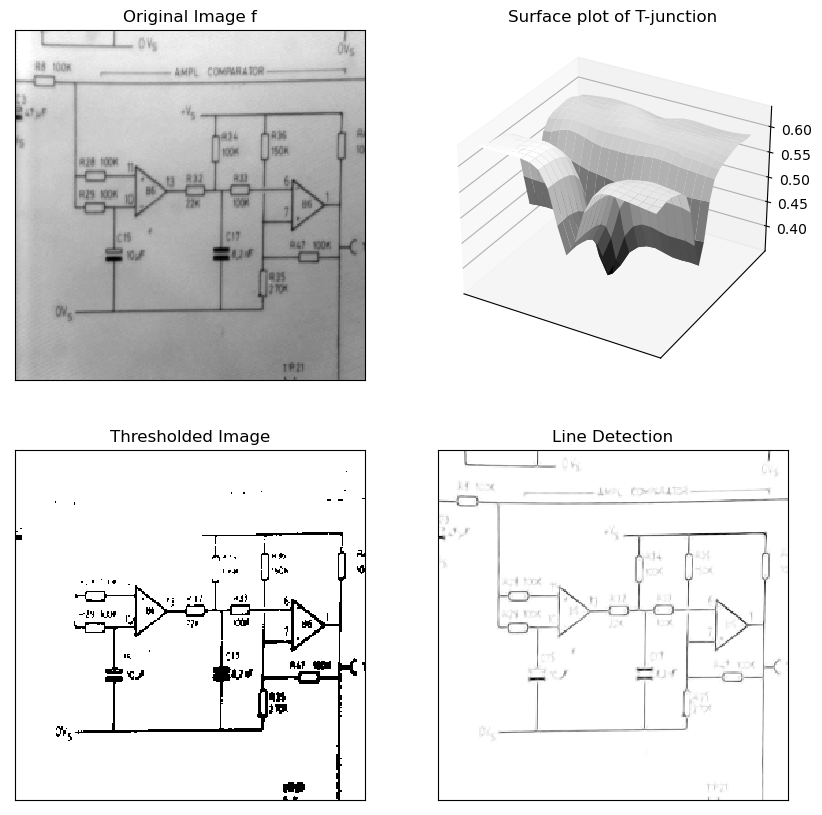
Fig. 6.23 Line Detection. In the top left an image of an electronic schematic. Goal is to detect the black lines. In the top right a surface plot of a small detail from the image showing a T-junction of lines. The lines show up as ‘gutters’ in the surface. The bottom of the gutters (where \(\nabla f\approx 0\)) are in the middle of the lines. Gutters are strongly curved in one direction and almost flat in the other direction. In the bottom left the original image after thresholding. Because of the uneven lighting over the image thresholding does not work. Lines in the top left of the image are missing. The bottom right shows the result of the line detector as discussed in this subsection.

A piece of a black line on a white background is a dark bar, i.e. characterized in the curvature gauge with

\[\begin{split}f_{pp} &\approx 0\\ f_{qq} &\gg 0\end{split}\]

and a vanishing gradient

\[f_w \approx 0\]

Combining the above three conditions can be done in a ‘fuzzy and’ expression:

\[\ell = \left( 1 - e^{-\frac{f_{qq}^2}{A}} \right)\; e^{-\frac{f_{pp}^2}{B}} \; e^{-\frac{f_w^2}{C}}\]

The first factor is approximately 1 in case \(f_{qq}\gg 0\), the second factor is approximately 1 in case \(f_{pp}\approx 0\) and the third factor is approximately 1 in case \(f_w\approx 0\). The product is therefore approximately 1 in case all three conditions are met with.

Footnotes

1

Mathematical the Njet characterized with derivatives up to order \(N\) is the equivalence class of all functions with the same derivatives (up to order \(N\)).