4. Geometrical Operators

An often used image operator is a geometrical operator, these are the operators that keep the colors the same but put the pixels in a different spot.

Image Warping

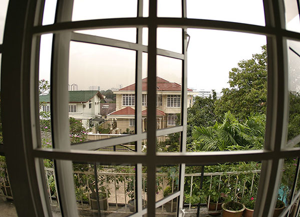
Optical Distorted Image

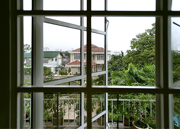
Corrected Image using Image Warping

These operators can be used to create some artistical effect, but they are also useful in correcting for some unwanted distortion, which were introduced, when the picture was taken (like camera rotation, perspective distortions etc.)

The input for these methods (at least in this Exercise) is always a quadrilateral region of a discrete image \(F\). That means that you only know the intensity values at discrete integral pixel positions. The output consists of a rectangular image \(G\) with axes aligned with the Cartesian coordinate axes \(x\) and \(y\).

In an arbitrary image transformation, there is no guarantee, that an “input”-pixel will be positioned at a pixel in the “output” image as well. Rather, most of the time your output image pixels will “look at” image positions in the input image, which are “between” pixels.

So you need access to intensity values, which are not on the sampling grid of the original image, e.g. the intensitiy value at position \((6.4, 7.3)\). In this section we assume that you know about interpolation. Here we focus on the basic structure of an image warping algorithm.

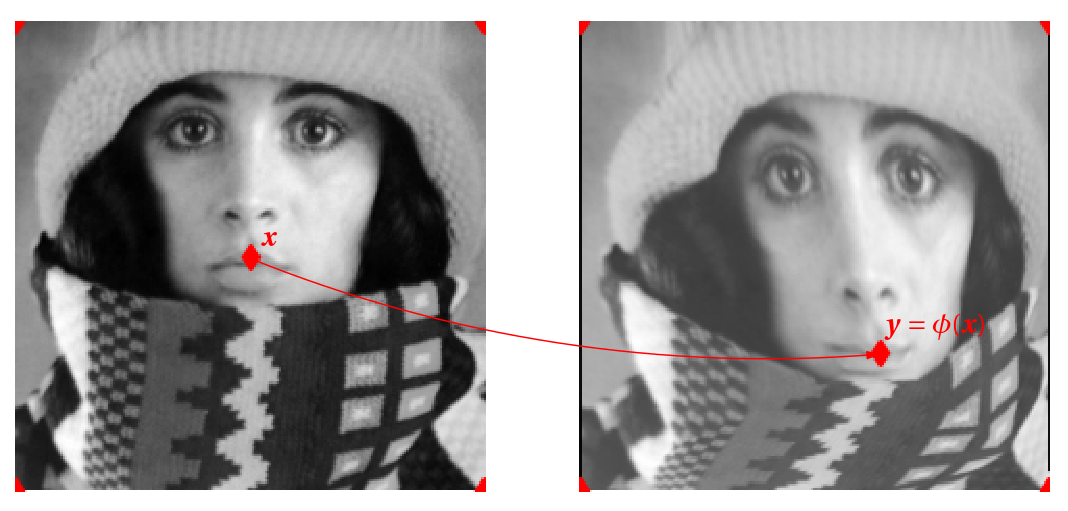
Fig. 4.1 Geometrical Operation. All points with their gray value (color value) in the image are put on a different spot. Indicated in the figure is that point \(\v x\) in the input image is ‘warped’ to position \(\v y =\phi(\v x)\) in the output image.

Let \(f\) be an image with domain \(E\) and range \(V\). Let \(\phi\) be a transform that takes a point \(\v x\in E\) and returns a point \(\v y=\phi(\v x)\) in the domain \(E'\) of image \(g\), we then define the geometrical transform \(\Phi\) as:

\[g(\v y) = (\Phi f)(\v y) = f(\v x)\quad\text{with}\quad \v y = \phi(\v x)\]

or equivalently:

\[g(\phi(\v x)) = f(\v x)\quad\text{or}\quad g(\v y) = f(\phi\inv(\v y))\]

in case the inverse transform exists.

Note that the last two transforms are equivalent from a mathematical point of view. We could start an algorithm for a geometrical operator with either equation. We start with the first one:

4.1. Forward Transform

import numpy as np
import matplotlib.pyplot as plt
from ipcv.ip.pixels import pixel, domainIterator;

def geoOp_fwd(f, phi):
   fdomain = f.shape[:2]
   g = np.zeros_like(f)
   for p in domainIterator(fdomain):
       q = phi(p).rint()
       if q.isin(fdomain):
           g[q] = f[p]
   return g

The function geoOp2d_fwd() is based on the first equation: we loop over all pixels in the domain of image \(f\), calculate where that pixel is transformed to and then set this pixel in the output image with the same color as the original pixel in the original image.

Below we define a function that rotates a pixel

def rotator(angle):
   ca = np.cos(angle)
   sa = np.sin(angle)
   R = np.array([[ca, -sa], [sa, ca]])
   def rotate(t):
       return pixel(R @ np.array(t))
   return rotate

and we use it to do an image rotation

Show code for figure

plt.figure(figsize=(10,5))

from ipcv.utils.files import ipcv_image_path
a = plt.imread(ipcv_image_path('peppers.png'));
plt.subplot(131); plt.imshow(a); plt.axis('off');
plt.title('Original');

b = geoOp_fwd(a, rotator(np.pi/6));
plt.subplot(132); plt.imshow(b); plt.axis('off');
plt.title('Rotated');

plt.subplot(133);
plt.imshow(b[:64,:64]);
plt.axis('off');
plt.title('Rotated (detail)');

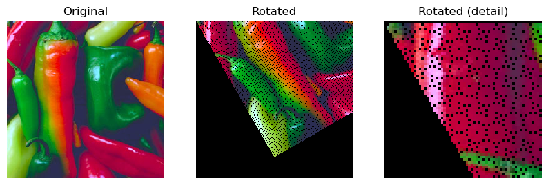
Fig. 4.2 Forward Geometrical Transform.

Evidently the forward transform is not the way to implement a geometrical transform. In the next sectio we will look at the backward transform that is based on the second formulation of the geometric operator.

4.2. Backward Transform

Instead of enumerating all pixels (sample positions) in the original image we now enumerate all pixels in the output image and use the inverse transform to calculate where that pixel came from in the original image.

def geoOp(f, invphi):
   g = np.zeros_like(f)
   gdomain = g.shape[:2]
   for q in domainIterator(gdomain):
       p = invphi(q).rint()
       if p.isin(gdomain):
           g[q] = f[p]
   return g

plt.subplot(131); plt.imshow(a);

b = geoOp(a, rotator(-np.pi/6))
plt.subplot(132); plt.imshow(b);
plt.subplot(133); plt.imshow(b[:64,:64]);

Fig. 4.3 Backward Geometrical Transform.

As can be clearly seen in this example the backward algorithm is the simplest one that really works. No more holes. Please note that we use a simple nearest neighbor interpolation. In practice it is much better to use a better interpolation scheme. Most image processing packages allow you to select one of several interpolation techniques.

4.3. Geometrical Transform in Scikit-Image

The most generic form of a geometrical transform is called skimage.transform.warp in skimage. As a second argument you have to pass it the inverse transform. It can be a function that takes an array of shape (M,2) of points in the result image and it should return an array of the shape giving the positions of the corresponding points in the input image. It is much like our geoOp function (only much faster). So let’s do the rotation again:

from skimage.transform import warp

def rotator_skimage(angle):
   ca = np.cos(angle)
   sa = np.sin(angle)
   RT = np.array([[ca, -sa], [sa, ca]]).T
   def rotate(x):
       return x @ RT
   return rotate

plt.subplot(131); plt.imshow(a); plt.title('Original')
c = warp(a, rotator_skimage(np.pi/6))
plt.subplot(132); plt.imshow(c); plt.title('Rotated')
plt.subplot(133); plt.imshow(c[:64,:64]); plt.title('Rotated (detail)')

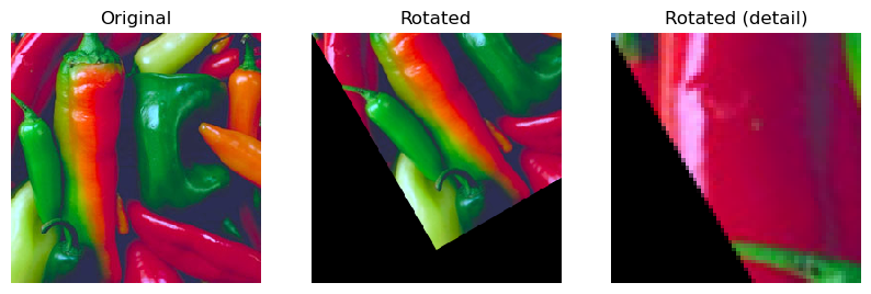
Fig. 4.4 Warp: Geometrical Transform in Scikit Image.

Scikit-Image has several functions for specialized geometrical transforms. In the example below we first set up the homogenuous matrix that rotates around the center of an image and then instead of using a callable as argument in warp we give it this matrix.

def rotation_matrix(f, angle):
   M,N = f.shape[:2]
   T = np.array([[1, 0, M/2],
                [0, 1, N/2],
                [0, 0, 1  ]])
   ca = np.cos(angle)
   sa = np.sin(angle)
   R = np.array([[ca, -sa, 0],
                 [sa,  ca, 0],
                 [ 0,   0, 1]])
   return T @ R @ np.linalg.inv(T)

plt.subplot(131); plt.imshow(a);
d = warp(a, rotation_matrix(a, np.pi/6))
plt.subplot(132); plt.imshow(d);
plt.subplot(133); plt.imshow(d[:64,:64]);

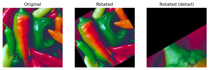
Fig. 4.5 Projective Geometrical Transform in Scikit Image.