6. Local Structure
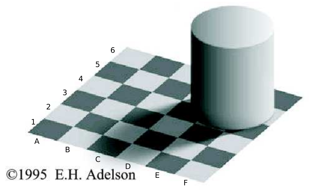
Fig. 6.1 Gray values “an sich” are not important. The tiles at B6 and D3 have exactly the same gray value.
The gray value (or color) value in a point, in isolation, is not essential in the interpretation of visual stimuli. Fig. 6.1 shows a famous example that illustrates this observation. The tiles at position B6 and D3 have exactly the same gray value. The visual information is encoded in the relation of the gray values in neighboring points in the image.
When looking at pictures, even abstract depictions of things you have never seen before, you will find that your attention is drawn to certain local features: dots, lines, edges, crossings etc. In a sense these are ‘prototypical pieces’ of an image, and we can describe every image as a field of such local elements. You may group these into larger objects and recognize those (i.e. assign semantic labels to the objects like ‘bike’ or ‘flower’ etc), but viewed as a bottom-up process perception starts with local structure.
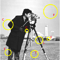
Fig. 6.2 Local Structure in images. In an image we distinguish several types of local structure like constant patches (F), edges (E), lines (L), corners (C) etc.
Note that the local structure patches in the image depicted in Fig. 6.2 are of different size (the encircled patches in the image). This is inevitable for any visual perception system looking at the 3D world. Objects that are further from the camera (or the eye in case of the human visual system) are depicted with smaller size in the image. When there is no a priori knowledge about the size (or scale) of the image details we are interested in, we need to analyze an image at all scales.
In fact at one point \(\v x\) in an image we may find different types of details at different scales (sizes). A constructed example is given in Fig. 6.3. At location \(\v x\) at small scale we ‘see’ the ending of a line whereas at larger scale the point \(\v x\) is a corner point. The fact that different types of details at different scales may be present at the same location can be seen in practice as well for instance when using the SIFT blob detector in scale space.
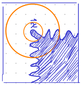
Fig. 6.3 Details at multiple scales.
In order to make the notion of local structure operational (i.e. computable) we have to define the notions of local and structure and make these quantifiable. In our exposition of local structure we will follow the lines of thought as pioneered by Jan Koenderink (a Dutch physicist who is world famous for his work on human perception, computer vision, geometry and color). He was one of the first, in the 80’s of the previous century, who combined the notion of scale and structure in a principled manner in which he stressed the fact that the structure of images reveals itself at all levels of details (resolution) simultaneously.
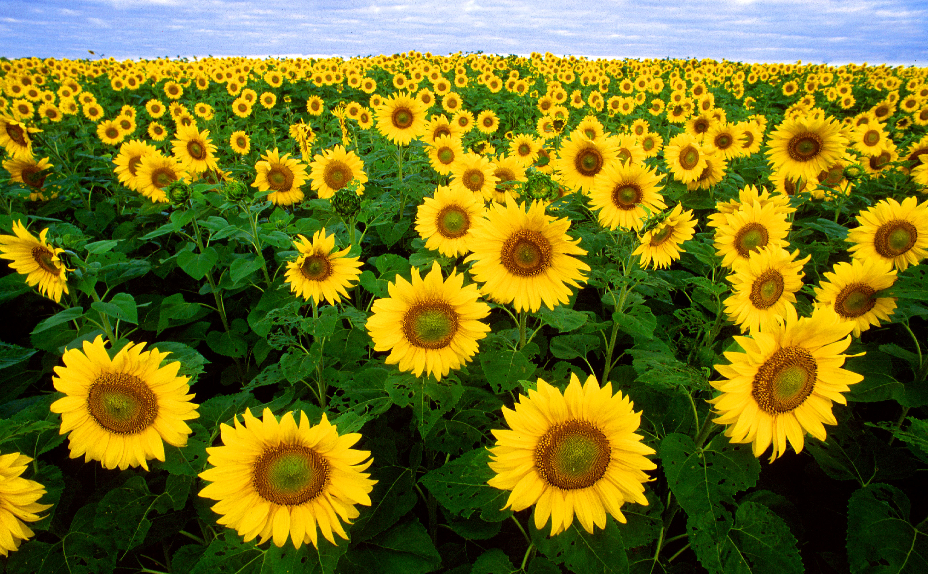
Fig. 6.4 Sunflowers.
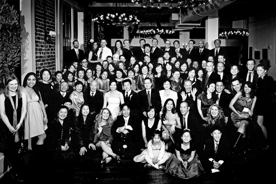
Fig. 6.5 Group portrait.
In Fig. 7.1 and Fig. 6.5 we see pictures that show blob like details (sunflowers and human faces) that are about the same size in the real world but are shown at different sizes in an image. To find these objects we must analyze the images at all levels of scale.
In a seminal paper The Structure of Images (1984) Koenderink argued that from basic principles (like translation invariance, rotation invariance and scale invariance) the most simple way to observe an image at all levels of resolution (scales) simultaneously is to embed the image into a one parameter family of images \(f(\v x, s)\):
For \(s>0\):
where \(f^0\) is the ‘zero scale’ image and the Gaussian kernel \(G^s\) is given by
We will also write \(f^s(\v x)=f(\v x, s)\). The zero scale image \(f^0\) is a mathematical abstraction, any observation of a physical quantity (like the light intensity) necessarily involves a probe of finite spatial and temporal dimension (see the section on image formation).
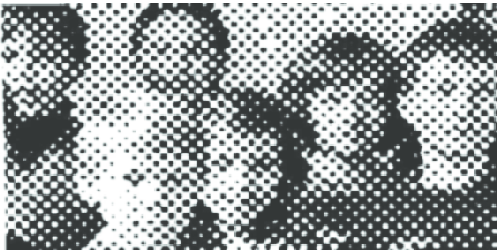
Fig. 6.6 Newspaper picture.
In Fig. 6.6 a picture as printed in a newspaper is shown. The printing process only uses black ink on white paper. The ‘illusion’ of gray values pops up in our brain when viewing the newspaper at such a distance that the human visual system blurs the image into a gray value version. That is why the image is rendered quite small on your screen. Click on the image to see a larger version where the ink blots are clearly visible.
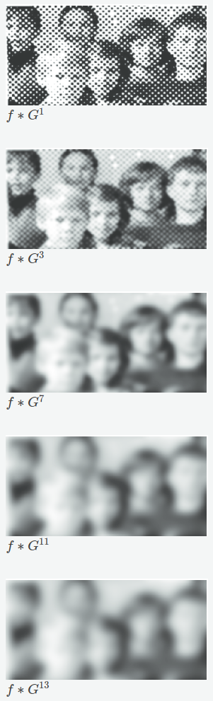
Fig. 6.7 Newspaper Scale-Space.
This blurring process can be done digitally as well and that is what is shown in Fig. 6.7. From the scale space of the newspaper image we can see that if we are interested in the original gray value image we should work with the image \(f\ast G^7\) instead of the original image \(f\). The printer on the other hand who looks for the sharpness and sizes of the individual ink blots is better off by looking at the original image (and indeed even looking at it through some magnifying glass).
The lesson to be learned is that there is no a priori ‘right scale’ to look for in an image. It depends not only on the size of the depicted objects visible in the image (like the sunflowers) but also on the goal of the observer (the printer versus the reader of a newspaper).
In this section on local structure we assume that enough a priori knowledge is available to select a fixed scale to observe the local structure. I.e. we select only one (or a few) scale(s) in the entire scale space. In the next chapter will build the entire scale space which we need in case there is no a priori knowledge about the scale/size of objects visible in the image that we are interested in.
In this chapter we will from here on concentrate on characterizing the local structure of images. Local in the sense that our characterization is valid in a small neighborhood of a point.
Modern deep learning methods learn the weight factors in convolution kernels from examples and the required result from the entire network. One needs very many learning examples to do this. It is however not too surprising that the results of those deep learning methods are very reminiscent of the local structure characterization that we will discuss in this chapter. This is true only for the very first layer in a deep network, the really novel part of deep learning networks is the way in which they are capable of combining the results from the lowest level to arrive at meaningful semantic labels for objects visible in an image.
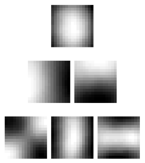
Fig. 6.8 Eigenimages as found with a principal component analysis of a set of small image details.
A very simple way to learn what types of neighborhoods are important for the visual system is by looking which local neighborhoods are most frequently occurring in natural images. It proves to be the case that the human visual system did just that: adapt itself to the visual stimuli that are omnipresent when looking at the world around us.
If you look at the set of all possible small images, say \(N\times N\) with \(N\) in the order of 16, all these examples can be considered to be data vectors in a 256 dimensional vector space. With a principal component analysis we can find a new set of basis vectors in the space corresponding with the directions with largest variance. Each of these basis vectors can then be viewed as a small image again. Any arbitrary image can then be written as a linear combination of those basis images. In case that detail image is from the same set of images than probably we need only a few of the 256 basis images (vectors) to represent that image without losing too much information. We then have described the local image structure (the \(16\times16\) image) with just a few numbers instead of the original 256 numbers.
In Fig. 6.8 the first six eigenimages from the PCA analysis of all small details in the ‘girl with sweater’ image are shown. The results are very similar with what we shall find with a more principled approach to be followed later in this chapter.
The local structure in a point \(\v x\) of an image will be characterized with the partial derivatives of the image \(f^s = f^0\ast G^s\). Remember from your math class that we can approximate a univariate function \(f\) in the neighborhood of a point \(a\) with its Taylor series approximation:
where we use \(f_x\) to denote the first order derivative of \(f\) with respect to \(x\), \(f_{xx}\) for the second order derivative etc.
When assessing the local structure of images we don’t consider the derivatives of the original image \(f\) but of the image observed at scale \(s\), i.e. \(f^s\). We then have:
For some functions the Taylor series (with infinite number of terms, i.e. derivatives of all orders) approaches the original function. In practice when using a Taylor series with a finite number of terms the approximation error is small only in a small neighborhood around the point \(a\) (where we have evaluated the derivatives). The neighborhood size is proportional to the scale \(s\).
Show code for figure
 1#
 2# Taylor Series of Smoothed Function
 3#
 4from matplotlib.pylab import *
 5
 6close('all')
 7
 8
 9def Gs(x):
10    return 1/(s*sqrt(2*pi)) * exp(-x**2/2/s**2)
11
12
13#x = arange(-100, 100)
14#f = sin(2*pi*x/100) + 0.2*sin(3*2*pi*x/100) + 0.3 * sin(5*2*pi*x/100)
15
16
17f = imread('source/images/trui.png')[128]
18x = arange(len(f))
19
20
21
22
23from scipy.ndimage import gaussian_filter
24from math import factorial
25
26idx_a = 100
27a = x[idx_a]
28N = 5 # Njet
29
30
31scales = [1,3,7,15]
32fig, axs = subplots(len(scales), 1, sharex=True, figsize=(8,8))
33
34for i, s in enumerate(scales):
35    axs[i].text(200, 0.6, f"scale (s) = {s}")
36
37    axs[i].plot(x, f, c='lightgray', linewidth=3, label=r'$f$')
38    fs = gaussian_filter(f, s)
39    axs[i].plot(x, fs, c='black', label=r'$f\ast G^s$')
40
41    fsa = zeros_like(fs)
42    for o in range(N+1):
43        fsa += 1/factorial(o) * (x-a)**o * gaussian_filter(f, s, o)[idx_a]
44
45
46    axs[i].plot(x, fsa, c='green', linewidth=2, label=r'Taylor approximation of $f\ast G^s$')
47
48    axs[i].set_ylim(f.min(), f.max())
49    axs[i].plot(x, f.min()+0.5*(f.max()-f.min())*Gs(x-a)/Gs(x-a).max(),
50                label=r'$G^s(x-a)$ (scaled to fit window)')
51    axs[i].axvline(a, c='gray', linestyle='dashed')
52    #axs[i].legend()
53
54
55handles, labels = axs[-1].get_legend_handles_labels()
56fig.legend(handles, labels, loc='upper left')
57savefig('source/images/smoothedtaylorapproximation.png')
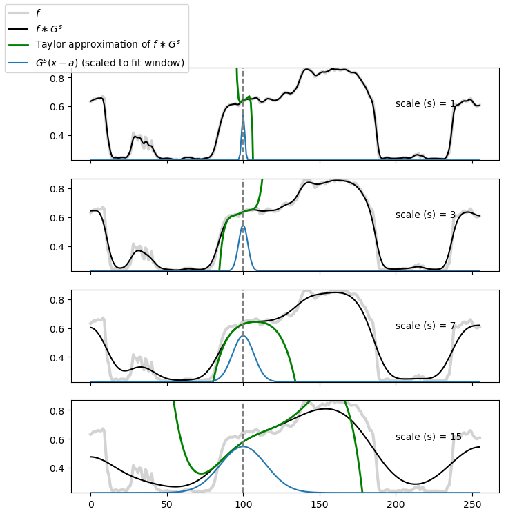
Fig. 6.9 Taylor Approximation for several scales. In light gray the original function \(f\) (in all subplots the same). In black the Gaussian smoothed image \(f\ast G^s\). In green the Taylor approximation (using up to the 5th order derivative) at \(a=100\). In blue the shifted (and scaled) Gaussian function \(G^s(x-a)\).
Observe in Fig. 6.9 that the Taylor approximation around \(a\) is close to the function \(f\ast G^s\) and the region in which the approximation is close is proportional with the scale \(s\). The scale of the Gaussian convolution thus indeed selects a scale that is proportional to the size of the neighborhood in which the local structure is characterized.
The derivatives or the Gaussian smoothed image \(f\ast G^s\) are not only useful to approximate the smoothed function but on their own they can be interpreted as measures that can be used to classify the neighborhood or to compare different neighborhoods on similarity. From a machine learning point of view the derivatives are a way to construct a representation of local neighborhoods with less data than the image neighborhood contains pixels.
In this chapter we will look at purely (differential) geometrical ways to characterize a neighborhood. The derivatives allow us to recognize a neighborhood as an edge between a dark and bright region, as a dark line on a bright background (or vice versa) or as a corner (and many more local geometry can be detected and localized in this way).
We also briefly describe a way to construct a statistical summary (histogram) of derivatives within a neighborhood. Just over 10 years ago these histograms of gradients were state of the art as the tool of choice to recognize objects in images.
But before we discuss local structure we start this chapter with a section on the Gaussian convolution \(f\ast G^s\) and the calculation of the partial derivatives of \(f\ast G^s\) (see Section 5.2).
Finally the sub pixel localization of local structure is discussed. In practical applications where accuracy is needed (e.g. when stitching images or when calibrating a camera) accurate localization of edges, lines and corners is important. It will be shown that these geometrical objects can be localized with far greater precision than the distance between two pixels in an image.