7.1. Linear Scale Space

Jan Koenderink

Prof. Jan Koenderink from Utrecht University formulated scale-space theory in the 1980’s. The seminal paper is: J.J. Koenderink, The Structure of Images, Biological Cybernetics, 1984. From the abstract: “In practice the relevant details of images exist only over a restricted range of scale. Hence it is important to study the dependence of image structure on the level of resolution. It seems clear enough that visual perception treats images on several levels of resolution.”

It may seem that there are enumerous ways to construct a scale-space. But surprisingly in case we set some simple requirements (basic principles) there is essentially only one scale-space construction possible.

Definition 7.1 ((Scale-Space Basic Principles))

We are looking for a family of image operators \(\op L^s\) where \(s\) refers to the scale such that given the ‘image at zero scale’ \(f^0\) we can construct the family of images \(\op L^s f^0\) such that:

1. \(\op L^s\) is a linear operator,

2. \(\op L^s\) is translation invariant (all parts of the image are treated equally, i.e. there is no a priori preferred location),

3. \(\op L^s\) is rotational invariant (all directions are treated equally, i.e. there is no a priori preferred direction),

4. \(\op L^s\) is separable by dimension, and

5. \(\op L^s\) is scale invariant (starting with a scaled version of the zero scale image we should in principle obtain the same scale-space with possible reparameterization of the scale).

It can be shown that the scale space operator satisfying all the requirements is the Gaussian convolution.

Theorem 7.2 (Linear Gaussian Scale-Space)

The scale-space operator that satisfies all basic principles is the Gaussian convolution:

\[f(\v x, s) = (f^0 \ast G^s)(\v x)\]

where \(G^s\) is the 2D Gaussian kernel:

\[G^s(\v x) = \frac{1}{2\pi s^2} \exp\left(-\frac{\|\v x\|^2}{2 s^2}\right)\]

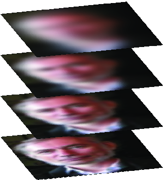
The function \(f\) can be interpreted as a one parameter family of images. For every scale \(s>0\) there is an image \(f(\cdot,s)\) that we will frequently refer to as \(f^s\).

Some properties of the Gaussian convolution (and hence of the linear Gaussian scale space construction) are already discussed in a previous chapter (see Section 6.1). For ease of reference we will repeat some of them here and state some more properties important in the scale-space context.

Theorem 7.3 (Linear Diffusion Equation)

The scale-space function \(f\) is the solution of the diffusion equation:

\[f_s = s \, \nabla^2 f = s (f_{xx}+f_{yy})\]

with initial condition \(f(\cdot,0)=f^0\).

In fact this differential equation was the starting point for Koenderink in deriving linear scale space (see linear_diffusion). From a practical point of view it is an important equation because it tells us that the change in the function \(f\) due to a small change in scale (going from scale \(s\) to scale \(s+ds\)) is proportional to the Laplacian differential structure of \(f\) at scale \(s\). It shows that in a Gaussian scale-space scale derivatives may always be exchanged for spatial derivatives.

Because taking a derivative is a linear translation invariant operator that commutes with the Gaussian convolution we have that any spatial derivative \(\partial_\ldots f\) adheres to the same scale space equation:

Theorem 7.4 (Scale Space Derivatives)

We can either first calculate a derivative and from that construct the scale-space or take the derivative at every scale in the scale-space:

\[\partial_\ldots f^0 \ast G^s = \partial_\ldots \left( f^0 \ast G^s \right)\]

where \(\partial_\ldots\) stands for any spatial derivnative. We can equivalently calculate the Gaussian derivative at all scales:

\[\partial_\ldots f^0 \ast G^s = f^0 \ast \partial_\ldots G^s\]

This theorem is a specific use of a more general theorem derivatives_of_convolution.

Show code for figure

#
# Normalized Gaussian Derivatives
#
import numpy as np
import matplotlib.pyplot as plt
from scipy.ndimage import gaussian_filter as gD
plt.close('all')

x = np.arange(0, 256)
f = 1.0 * (x>128)

fig_derivatives, axd = plt.subplots(2, 2, sharex=True, figsize=(10,10))

axd[0, 0].plot(x, f, label="f")
axd[0, 1].plot(x, f, label="f")
for s in np.logspace(1, 1.5, 10):
    fx = gD(f, s, 1)
    axd[0, 0].plot(x, fx, label=f"s = {s:2.2f}")

    fxx = gD(f, s, 2)
    axd[0, 1].plot(x, fxx, label=f"s = {s:2.2f}")


axd[0, 0].set_ylim(0, 0.05)
axd[0, 1].set_ylim(-0.0030, 0.003)
axd[0, 0].set_title(r"$f\ast G_x^s$")
axd[0, 1].set_title(r"$f\ast G_{xx}^s$")


axd[1, 0].plot(x, f, label="f")
axd[1, 1].plot(x, f, label="f")
for s in np.logspace(1, 1.5, 10):
    fx = gD(f, s, 1)
    axd[1, 0].plot(x, s * fx, label=f"s = {s:2.2f}")

    fxx = gD(f, s, 2)
    axd[1, 1].plot(x, s**2 * fxx, label=f"s = {s:2.2f}")


handles, labels = axd[0,0].get_legend_handles_labels()
fig_derivatives.legend(handles, labels, loc='upper left')
axd[1, 0].set_ylim(0, 0.5)
axd[1, 1].set_ylim(-0.3, 0.3)
axd[1, 0].set_title(r"$s (f\ast G_x^s)$")
axd[1, 1].set_title(r"$s^2 (f\ast G_{xx}^s)$")



fig_flower, axf = plt.subplots(2, 5, figsize=(10,5))
try:
    f = plt.imread('../../source/images/flowers.jpg')
except:
    f = plt.imread('source/images/flowers.jpg')

x, y = 40, 90
w, h = 150, 150
f = f[y:y+h, x:x+w, 1]/255
axf[0, 0].imshow(f, cmap=plt.cm.gray)
axf[0, 0].axis('off')
axf[1, 0].imshow(f, cmap=plt.cm.gray)
axf[1, 0].axis('off')

for i, s in enumerate(np.logspace(0, 1, 4)):
    #fw = np.hypot(gD(f, s, (0, 1)), gD(f, s, (1, 0)))
    fx = gD(f, s, order=(0, 1))
    fy = gD(f, s, order=(1, 0))
    fw = np.hypot(fx, fy)
    axf[0, i+1].imshow(fw, cmap=plt.cm.gray, vmin=0, vmax=0.3)
    axf[0, i+1].set_title(f"s = {s:2.2f}")
    axf[0, i+1].axis('off')

    axf[1, i+1].imshow(s * fw, cmap=plt.cm.gray, vmin=0, vmax=0.3)
    axf[1, i+1].axis('off')

fig_flower.tight_layout()
    

fig_grad_flower, axs = plt.subplots(2, 2, figsize=(5,5))

color = "orange"
x, y = 30, 95
w, h = 32, 32
f = f[y:y+h, x:x+w]

f1 = gD(f, 1, 0)
f4 = gD(f, 4, 0)
axs[0,0].imshow(f1, cmap=plt.cm.gray)
axs[0,1].imshow(f4, cmap=plt.cm.gray)


fx1 = gD(f, 1, (0,1))
fy1 = gD(f, 1, (1,0))
fw1 = np.hypot(fx1, fy1)
axs[1, 0].imshow(fw1, cmap=plt.cm.gray)

xp, yp = 14, 19
L = 20

fxp = fx1[yp, xp]
fyp = fy1[yp, xp]
axs[1,0].arrow(xp, yp, L * fxp, L * fyp, width=0.5, color=color)
axs[0,0].arrow(xp, yp, L * fxp, L * fyp, width=0.5, color=color)

fx4 = 4 * gD(f, 4, (0,1))
fy4 = 4 * gD(f, 4, (1,0))
fw4 = np.hypot(fx4, fy4)
axs[1, 1].imshow(fw4, cmap=plt.cm.gray)

fxp = fx4[yp, xp]
fyp = fy4[yp, xp]
axs[1,1].arrow(xp, yp, L * fxp, L * fyp, width=0.5, color=color)
axs[0,1].arrow(xp, yp, L * fxp, L * fyp, width=0.5, color=color)

for ax in axs.flatten():
    ax.axis('off')

axs[0,0].set_title(f"$f^1$")
axs[0,1].set_title(f"$f^4$")
axs[1,0].set_title(f"$f_w^1$")
axs[1,1].set_title(f"$f_w^4$")
fig_derivatives.savefig('source/images/derivatives_step.png')

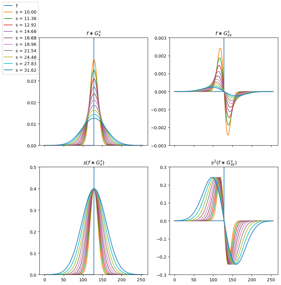
Fig. 7.2 (Normalized) Gaussian Derivatives of Step Function. On the first row the first order (left) and second order (right) derivative of a step function. On the second row the normalized first and second order derivatives.

In Fig. 7.2 we show a step function and its first and second order derivatives calculated at several scales in the top row. It is evident that the derivatives decrease in amplitude with increasing scale. When comparing derivatives accross scale this is problematic. To solve this problem we will use scale normalized derivatives.

Definition 7.5 (Scale Normalized Derivatives)

Let \(\partial_\ldots^k\) denote any \(k\)-th order spatial derivative than the scale normalized Gaussian spatial derivative is given as:

\[s^k (f^0 \ast \partial_\ldots^k G^s)\]

The scale normalized derivatives for the step edge are shown in in the bottom row of Fig. 7.2.

Show code for figure

# see code for a previous figure
fig_flower.savefig('source/images/flower_gradient.png')

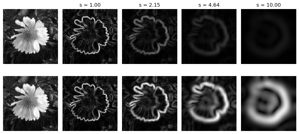
In Fig. 7.3 the standard derivatives are compared with the normalized derivatives. On the first row first the original image followed by \(f^s_w\) (the gradient norm) for several values of the scale \(s\). On the second row again the original image but now with the normalized gradient \(s f^s_w\).

Show code for figure

# see code for a previous figure
fig_grad_flower.savefig('source/images/fig_flower_gradient_vector.png')

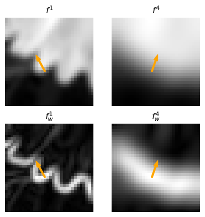
Fig. 7.4 Gradient Vector dependent on scale.

The images of the flower show that the gradient calculated in one point is dependent on the scale of the Gaussian convolution. In Fig. 7.4 we see a small detail of the flower. In the left column the scale is \(s=1\), where in the top row we see the image \(f^1\) and in the bottom row \(f^1_w\). Also shown is the gradient vector \(\nabla f^1\) in one point in the image. In the right column the scale is \(s=4\). Observe the change in direction of the gradient vector when compared with the gradient at scale \(s=1\).

When constructing a scale-space we can calculate each scale by convolving the zero scale image. But given the semi group property of the Gaussian convolution (see Proof 6.4) the scale space can be constructed incrementally. For ease of reference we repeat that theorem here:

Theorem 7.6 (Semi Group of Gaussian Convolutions)

If we take a Gaussian function \(G^s\) and convolve it with another Gaussian function \(G^t\) the result is a third Gaussian function:

\[G^s \ast G^t = G^{\sqrt{s^2+t^2}}\]

So given the image \(f^s\) the image at scale \(t\) (with \(t>s\) can be calculated as:

\[f^t = f^0 \ast G^t = f^s \ast G^{\sqrt{t^2-s^2}}\]

The computational complexity of the Gaussian convolution \(f\ast G^s\) is proportional to the scale \(s\). So the calculation is \(\bigO(t)\). The computational complexity of the calculation \((f\ast G^s)\ast G^\sqrt{t^2-s^2}\) is \(\bigO(s+\sqrt{t^2-s^2})\). It is not too difficult to prove that in general \(\bigO(s+\sqrt{t^2-s^2}) < \bigO(t)\). However, although incrementally building a scale space is more efficient it is not always to be preferred because Gaussian convolutions at small scales are always less accurate than convolutions at larger scale.

In Section 7.3 we will look at constructing scale-space from a discrete, i.e. sampled image.