3.1. Image Arithmetic

Show code for figure

import numpy as np
import matplotlib.pyplot as plt
from ipcv.utils.files import ipcv_image_path

plt.close('all')

a = plt.imread(ipcv_image_path('cermet.png'))
b = plt.imread(ipcv_image_path('trui.png'))

plt.subplot(131);
plt.title('a',size='xx-small');
plt.imshow(a);
plt.axis('off');
plt.subplot(1,3,2);
plt.title('b',size='xx-small');
plt.imshow(b);
plt.axis('off');
plt.subplot(1,3,3);
plt.title('(a+2*b)/3',size='xx-small');
plt.imshow((a+2*b)/3);
plt.axis('off');
plt.subplots_adjust(hspace=0.3, wspace=0.05);

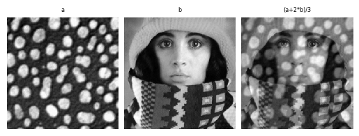
Fig. 3.2 Image Arithmetic.

Consider two 2-dimensional images \(f\) and \(g\) both with signature \(\setR^2\rightarrow\setR\) and both sampled on the same grid resulting in discrete representations \(F\) and \(G\) respectively. The point wise addition of the two images \(h=f+g\) is defined by:

\[\forall \v x\in\setR^2: h(\v x) = (f+g)(\v x) = f(\v x) + g(\v x)\]

When we sample the addition of the two images on the same grid \(B\) we obtain the discrete image \(H\):

\[\forall \v k \in\setZ^2: H(\v k) = F(\v k) + G(\v k)\]

The Python code for the addition of two images is:

# Addition of two images
def addImage(f, g):
  h = f.copy()
  for p in domainIterator(f):
    h[p] = f[p] + g[p]
  return h

Python Programming

The copy of f to make the output image h is an easy way to be sure that the output image is of the same size and type as the input image. Please note that there is no checking on what size and type image g is (in production code this is needed of course).

Also note that a multi dimensional array in Numpy may be indexed with a[p] in case p is a tuple of integers. The function domainIterator returns an iterator that returns the tuples of all multi-indices in the image domain.

In the above example we have lifted a well defined operator (the scalar addition \(+\)) to work on images by applying it pairwise to all pixels of the two images. Consider again the definition of the image addition operator \((f+g)(\v x) = f(\v x) + g(\v x)\). The operator \(+\) in the left hand side working on images is defined in terms of the operator working on scalars at the right hand side.

The addition of two images in terms of a pixel wise addition of the pixel values is not needed in Python. Python automatically lifts many of the standard arithmetic operators to work on images (i.e. arrays). The addition of the two images f and g can be simply written as f+g.

3.1.1. Definition

More formally we can repeat this lifting procedure for any scalar function \(\gamma\). Consider two images \(f:\set D\rightarrow \set R\) and \(g:\set D\rightarrow \set R'\). Let \(\gamma:\set R\times \set R'\rightarrow \set R''\) be an operator that takes a value from \(\set R\) and a value from \(\set R'\) and produces a value from \(\set R''\). Such a binary operator \(\gamma\) can be lifted to work on images:

\[\forall\v x\in \set D: \gamma(f,g)(\v x) = \gamma( f(\v x), g(\v x) )\]

Note that the \(\gamma\) function on the right hand side working on the image values is assumed to exist and that the \(\gamma\) working on images is defined through the above equation. An image operator constructed by pointwise lifting a value operator to the image domain is called a point operator. We will implicitly assume such a lifting construction when we talk about the addition, subtraction, multiplication etc. of images.

We will write \(\gamma\) when operating on image values and images alike. Effectively we are overloading the \(\gamma\)-function to work on both values and images.

Many of the common binary operators on real numbers are written in an infix notation (like \(f+g\), \(f-g\), etc). We will follow that convention and write \(f+g\) to denote the point wise addition of two images.

The lifting construction of a point operator is easily discretized. Let \(F\) and \(G\) be the sampled discretizations of the images \(f\) and \(g\) respectively. The discretization \(H\) of the image \(h=\gamma(f,g)\) is:

\[H(k) = \gamma( F(k), G(k) )\]

This shows that we can define the discrete image operator \(\Gamma\) working on discrete image representations \(H = \Gamma(F,G)\). For lifted point operators we never will make the distinction between \(\gamma\) and its discretized version \(\Gamma\) again.

3.1.2. Python/Numpy

In Python/Numpy the idea of lifting operators from their definition working on scalars to work on images (ndarrays in Numpy) is elegantly implemented using the idea of universal functions (as quoted from the documentation):

“A universal function (or ufunc for short) is a function that operates on ndarrays in an element-by-element fashion, supporting array broadcasting, type casting, and several other standard features.”

The term “type casting” refers to the mechanism for automatical type conversion in case the operator requires so. The term “array broadcasting” refers to the mechanism to adapt and set the dimensions of the operands. Array broadcasting is the mechanism that allows us to write f+1 where f is an image (ndarray). The result is that 1 is added to all elements of f.

For an overview of all point operators (or universal functions in Numpy speak) we refer to the Numpy documentation

3.1.3. Practical Use

3.1.3.1. \(\alpha\)-Blending

Show code for figure

from ipcv.utils.files import ipcv_image_path

f = plt.imread(ipcv_image_path('cermet.png'))
g = plt.imread(ipcv_image_path('trui.png'))
N = 5
alph = np.linspace(0,1,N)

for i in range(N):
    a = alph[i]
    plt.subplot(1,N,i+1)
    plt.title("%2.2f" % a, size='xx-small')
    plt.imshow((1-a)*f+a*g)
    plt.axis('off')

plt.subplots_adjust(hspace=0.3, wspace=0.05)

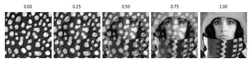
Fig. 3.3 Alpha Blending of two images.

Point operators, although very simple, are often used in practical applications of image processing. A simple example is the weighted average of two images. Let \(f\) and \(g\) be two color images defined on the same spatial domain. A sequence of images that shows a smooth transition from \(f\) to \(g\) (if rendered as a movie) is obtained by:

\[h_\alpha = (1-\alpha) f + \alpha g\]

for \(\alpha\) values increasing from 0 to 1. Such a sequence (for a grey scale image) is depicted above. The Python code to generate the \(\alpha\)-blend of two images is:

# Alpha blending of two images
def alphaBlend(f, g, alpha):
  return (1 - alpha) * f + alpha * g

3.1.3.2. Unsharp Masking

Show code for figure

from scipy.ndimage.filters import gaussian_filter
from ipcv.utils.files import ipcv_image_path

f = plt.imread(ipcv_image_path('trui.png'))
g = gaussian_filter(f, 3)
h = f + 3*(f-g)
plt.figure(1);
plt.subplot(131);
plt.imshow(f, vmin=0, vmax=1);
plt.title('f', size='xx-small');
plt.axis('off');
plt.subplot(132);
plt.imshow(g, vmin=0, vmax=1);
plt.title('g',size='xx-small');
plt.axis('off');
plt.subplot(133);
plt.imshow(h, vmin=0, vmax=1);
plt.title('f+3*(f-g)',size='xx-small');
plt.axis('off');
plt.subplots_adjust(hspace=0.3, wspace=0.05);

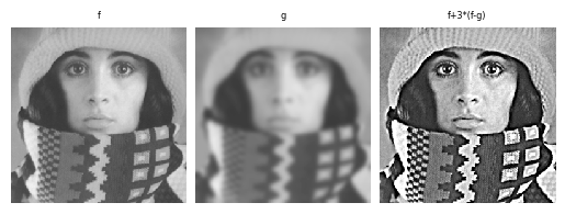
Fig. 3.4 Unsharp Masking.

A second example using alpha blending of two images is unsharp masking. This technique takes an image \(f\) and a blurred version of that image (we call it \(g\)). The result image then is obtained by adding \(\beta\) times the difference \(f-g\) to the original image:

\[h = f + \beta(f-g)\]

For some more background on the origin of unsharp masking we refer to the article on Wikipedia.

In a later chapter we will learn how to blur an image through Gaussian convolution, only then we can understand why this seemingly weird operation is capable of sharpening the image.

3.1.3.3. Thresholding

An example of the use of a relational operator (resulting in a boolean or binary image) is image thresholding. Let \(f\) be a scalar image, than \(\left[f>t\right]\) (for constant \(t\)) results in a binary image. Note that in Numpy the explicit use of the Iverson brackets are not needed.

Show code for figure

from ipcv.utils.files import ipcv_image_path

f = plt.imread(ipcv_image_path('rice.png'))[:,:,1] # only the green component
b = f>0.45
plt.figure(1);
plt.subplot(1,2,1);
plt.imshow(f,cmap='gray');
plt.axis('off');
plt.title('f');
plt.subplot(1,2,2);
plt.axis('off');
plt.imshow(b,cmap='gray');
plt.title('f>0.45');

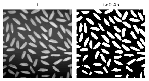
Fig. 3.5 Image Thresholding.

The traditional interpretation of such a binary image is of white objects (the 1 pixels) against a black background (the 0 pixels).

3.1.4. Exercises

1. Blending Color Images. In case we have an operator \(\gamma\) defined on two color values we can obviously lift this operator to work on color images as well. In case the operator \(\gamma\) itself is the ‘lifted’ version of an operator working on scalars then Python/Numpy is of great help. E.g. the addition of two color images is the component-wise addition (i.e. adding red, green and blue components independently) can be simply done with f+g. Implement the \(\alpha\)-blend of two color images.

2. Unsharp Masking.

   1. Show that unsharp masking of an image \(f\) is equivalent to alpha blending of the image \(f\) and a smoothed version \(g\) of \(f\). What is the \(\alpha\) factor in this case (as a function of \(\beta\)).

   2. For each of the images \(f\), \(g\) and \(f-\beta(f-g)\) from the example previously shown also plot the grey profile along a horizontal line through the center of the image (i.e. plot f[128,:]). This plot reveals why unsharp masking ‘sharpens’ an image.

3. Unsharp Masking of Color Images. Implement an algorithm for the unsharp masking of color images. There is no unique way to do this. You could first transform the image to a color model that explicitly encodes the luminance (brightness or value) and two color coordinates. Then operate on the luminance channel only. Or you could just work on the red, green and blue image independently. Comment on your findings comparing both versions.