1.6. Image Representation

1.6.1. Coordinates and Indices

Accustomed to the choice of coordinate axes in mathematics you might think that the axes for an image \(f(x,y)\) are the same: the x-axis running from left to right, the y-axis from bottom to top with the origin in the lower left corner. This is not true for digital images in general (the one exception i know of is Microsofts Device Independent Bitmap).

In order to get an understanding of the many different formats for digital images we have to distinguish:

• the axes with the coordinates along those axes, and

• the indices into the array representing all samples.

We will use numpy and matplotlib throughout to set our definition for these lecture notes.

We will use this image \(f\) as leading example:

\[\begin{split}\begin{array}{cccc} 0& 1& 2& 3\\ 4& 5& 6& 7\\ 8& 9&10&11 \end{array}\end{split}\]

In numpy this is easy to generate and plot with matplotlib:

Show code for figure

f = np.arange(12).reshape(3,4)
plt.imshow(f, cmap='gray', interpolation='nearest');

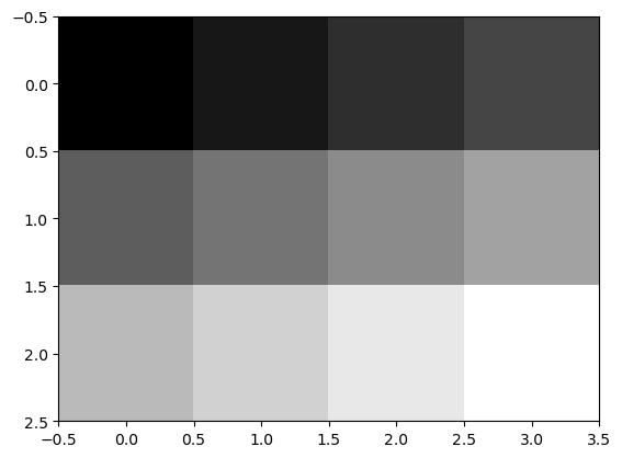
Fig. 1.17 Image Axes.

The sample points are in the middle of the squares (NOT pixels) and we see that the origin with coordinates is chosen to be at the top left. The x-coordinate axis runs from left to right and the y-coordinate axis runs from top to bottom.

In this coordinate axes system we can draw a line from \((0,2)\) to \((3,0)\). Being familiar with numpy arrays you have probably understood that in case we want to index the array with the coordinates \((x,y)\) (with \(x\) and \(y\) integer valued of course) that we need to write f[y,x].

Show code for figure

f = np.arange(12).reshape(3,4)
plt.imshow(f, cmap='gray', interpolation='nearest');
plt.plot([0,3], [2,0], lw=3);
plt.savefig('source/images/imageaxesplot.png')

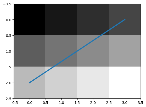
Fig. 1.18 Line plotted on top of image.

Carefully note that the coordinate system is a left-handed one. You have to turn the x-axis clockwise to the y-axis. The classical choice with x axis from left to right and y-axis from bottom to top results in a right-handed coordinate system. Be aware that in a left handed system things are a bit different than you might expect. A rotation over a positive angle \(\phi\) characterized with rotation matrix:

\[\begin{split}R = \matvec{cc}{\cos\phi & -\sin\phi\\ \sin\phi & \cos\phi}\end{split}\]

is turning a vector counter clockwise in a right handed coordinate system, but clockwise in a left handed system.

So, the first index in the image array is the y-coordinate, and the second index is the x-coordinate.

1.6.2. Color Images

Let’s read a color image from disk and display it:

Show code for figure

f = plt.imread(ipcv_image_path('peppers.png'))
plt.imshow(f);
print(f"f.shape = {f.shape}")

f.shape = (256, 256, 3)

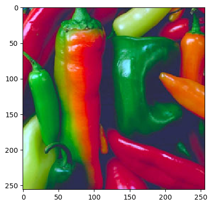
Fig. 1.19 RGB color image represented as \(M\times N\times 3\) array.

The shape of a color image array thus is \(M\times N \times 3\). It is also possible that a 4-th channel is used that encodes the transparency mask when displaying an image. Be sure to check and not assume things that are not nescessarily true.

A note of warning. Most often the channels in a color image are

R,G,B. A noteworthy exception is the OpenCV package where the channel sequence is B,G,R.

Each of the planes f[:,:,c] with c equal to 0, 1 or 2 gives one of the color planes. Each color plane is a scalar image and can be displayed as such:

Show code for figure

plt.imshow(f[:,:,1], cmap='gray');

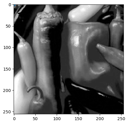
Fig. 1.20 Green channel of color image is a reasonable approximation of the luminance of a color image.

1.6.3. Domain Iterators

A lot of image processing algorithms are of the form: for every pixel in the image make a calculation and assign the calculated value to the corresponding pixel in the output image.

In Python/Numpy that is easy to do:

def negateImage(image):
  result = empty(image.shape)
  for p in domainIterator(image.shape):
    result[p] = 1 - image[p]
  return result

In the above code a simple point operator is implemented: the negation (negative) of an image, assuming the range of the image is \([0,1]\in\setR\).

The domain iterator enumerates all pixels in the image as index tuples. Here we make use of the fact that in case a is a Numpy array we may index this multidimensional array as a[p] in case p is \(n\)-tuple where \(n\) is the dimension of the image.

Show code for figure

f = np.arange(12).reshape((3, 4))
plt.imshow(f, cmap='gray', interpolation='nearest');
pts = np.array(list(domainIterator(f.shape)))
plt.plot(pts[:,1], pts[:,0], 'or');
for i, (p,dp) in enumerate(zip(pts[:-1], pts[1:] - pts[:-1])):
    plt.arrow(p[1], p[0], dp[1], dp[0], width=0.01, color='blue')
    plt.text(p[1] + 0.2, p[0] - 0.2, str(i), color='green')
plt.text(pts[11,1] + 0.2, pts[11,0] - 0.2, str(11), color='green');
plt.title('Raster Scan Iterator');

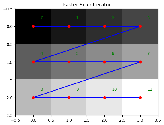
Fig. 1.21 Raster Scan Iterator.

For a two dimensional image enumerating all indices is easy. In Python we can write the domain iterator based on the generator concept using the yield statement.

def domainIterator2D(size):
  for i in xrange(size[0]):
    for j in xrange(size[1]):
      yield (i,j)

Because the statement yield is used this function behaves like an iterable. for p in domainIterator2D(image.shape): will do the job in the negateImage function.

The approach discussed requires us to write iterators for all dimensions we are interested in. We would like to define a function that can be used for all possible dimensions. The following generator (function using yield) does just that.

def domainIteratorND(size):
  """
  Return an iterator that yields the multidimensional indices as
  tuples within the interval (0)-(size)
  """
  index = zeros(len(size))
  for i in xrange(prod(size)):
    yield tuple(index)
    carry = 1
    for k in xrange(len(size)):
      if index[k]+carry >= start[k]+size[k]:
        index[k] = start[k]
      else:
        index[k] += 1
        break

Python has built in functions to make the above about twice as fast. It uses the product function from the itertools module. This product is the Cartesian product of sets (generate all combinations taking 1 element from each of the sets). It is essentially a one-liner function but with some extra lines to deal with parameters.

ipcv.ip.pixels.domainIterator(end, start=None, step=None)

Returns an iterator that yields all multi-indices in the range (start)-(end) with stepsizes (step) in rasterscan order

def domainIterator(end, start=None, step=None):
    """
    Returns an iterator that yields all multi-indices in the range
    (start)-(end) with stepsizes (step) in rasterscan order
    """
    if type(end) != ndarray:
        end = array(end);
    if start == None:
        start = 0*end;
    elif type(start) != ndarray:
        start = array(start)
    if len(start) != len(end):
        raise IPCVError("start and end should have same length")
    if step != None and type(step) != ndarray:
        step = array(step)

    if step == None:
        return product(*[ arange(*p) for p in zip(start, end) ])
    else:
        return product(*[ arange(*p) for p in zip(start, end, step) ])

We have given only a raster scan iterator over a (sub) image domain. In practice we need more than that:

• rasterscans in different orders (forward and reverse) and in different axes combinations (any permutation of the axes will give a valid scan of all pixels in the image).

• scans based on image content (e.g. enumerate all pixels with value greater than or equal to a given value, or all pixels on the border of an object, or all pixels connected to a given pixel, or…).

Although image processing as part of computer science exists since the 1960-ties there is still no widely accepted STL (Standard Template Library: C++ template for standard data structures and algorithms) type of iterator and algorithm library (although there are a lot of efforts). Ideally we would like a way to express our image processing algorithms (our condensed knowledge) in a form (code/specification) that can withstand time and new programming languages and computer architectures.