1.3. Image Discretization
To store an image function \(f: \setR^d \rightarrow \setR\) in computer memory we need to make a discrete representation of it. Image discretization involves two separate processes: discretization of the spatial domain (sampling) and discretization of the image range (quantization).
1.3.1. Quantization
The classical grey value image is a mapping from the spatial domain \(\setR^2\) to the set of luminance values \(\setR\). These luminance values are always positive (there is no such thing as a negative energy that can be observed). Luminances are also restricted to a finite range. There is an energy level that completely saturates the image sensor, such that no larger luminance levels can be observed. Traditionally the luminance range is encoded in 256 levels from 0 to 255, corresponding with an 8 bit discretization of the luminance range. Nowadays grey value luminance ranges are encoded in some sensors in up to 12 bits (especially for medical X-ray images). Color images are most often represented using an 8 bit encoding of the red, green and blue channel each (making up a 24 bit per pixel encoding of the image).
We will always assume that the image is properly quantized, meaning that it does not only allow for a faithful representation of the observation but that it also facilitates the necessary image computations. In practice this is dependent on the both the images (CT images have a luminance range that needs more than 10 bits for proper discretization whereas your cheap web-cam only needs about 6 bits (for each of the 3 color channels)) as well as on the type of computations needed (calculating the gradient, based on first order derivatives, requires negative numbers).
Word of advice: when developing image processing algorithms start with images quantized with floating point values. Only when speed and or memory is important look for other (integer valued) representations. You would not be the first to be bewildered by the difference in results of image expressions like
g = (f - f.min()) / (f.max()-f.min()) * 255
h = 255 * (f - f.min()) / (f.max()-f.min())
Show code for figure
 1import numpy as np
 2import matplotlib.pyplot as plt
 3from skimage.io import imread
 4from ipcv.utils.files import ipcv_image_path
 5
 6f = imread(ipcv_image_path('trui.png'))
 7g = (f - f.min()) / (f.max()-f.min()) * 255
 8h = 255 * (f - f.min()) / (f.max()-f.min())
 9plt.figure(figsize=(10,4))
10plt.subplot(131);
11plt.imshow(f);
12plt.axis('off');
13plt.title(f"f ({f.dtype})");
14plt.subplot(132);
15plt.imshow(g);
16plt.axis('off');
17plt.title(f"g ({g.dtype})");
18plt.subplot(133);
19plt.imshow(h);
20plt.axis('off');
21plt.title(f"h ({h.dtype})");
22plt.savefig('source/images/uintcalculations.png')
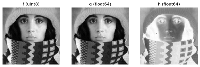
Fig. 1.8 Calculation with uint8 image leading to unexpected results.
1.3.2. Sampling
In a previous section on image formation we have seen that an image can only be observed in a finite number of, sample, points. The set of sample points is called the sampling grid. In these notes we assume a simple rectangular sampling grid restricted to a rectangular subset of the plane.
In some situations we need to distinguish between image functions defined on a continuous domain (i.e. \(\setR^2\)) and discrete, i.e. sampled images. In such situations we will often use lower case letters for the images with a continuous domain and uppercase letters for sampled images.
The image \(f:\setR^2\rightarrow\setR\) is sampled to obtain the function \(F\) defined on a discrete domain \(F:\setZ^2\rightarrow\setR\):
where \(\Delta x\) and \(\Delta y\) are the sampling distances along the \(x\) and \(y\) axis respectively.
The mathematical notion of sampling is a theoretical abstraction. It assumes an image function can be measured in a mathematical point (with no area). In practice a sample is always some kind of average over a small area (most often a rectangular part of the CCD or CMOS chip in case of optical or X-ray imaging).
A pixel stands for a picture element.
Show code for figure
1import numpy as np
2import matplotlib.pyplot as plt
3plt.close('all')
4f = np.arange(12).reshape(3, 4)
5k, l = np.meshgrid(np.arange(4), np.arange(3))
6plt.imshow(f, interpolation='nearest', cmap='gray');
7plt.scatter(k, l, s=100, c='g');
8plt.savefig('source/images/pixel_samples.png')
Fig. 1.9 A rectangular image of 12 pixels in total. The sample positions (pixel positions) are indicated as green points overlayed on the standard image display). Note that the sample positions have integer value coordinates. But also note that on the screen the pixel value \(F(i,j)\) is used to fill the square \(i-0.5<k<i+0.5\), \(j-0.5<l<j+0.5\) for the screen pixels with coordinates \((k,l)\).
Unfortunately many people think of images as being composed of these small little squares (the pixels) each with uniform color. Despite the fact that images can and are often displayed like this as shown in Fig. 1.9 thinking the pixels are little squares is wrong however: A pixel is not a little square. Remember: A pixel is a point sample and an image is a regular grid of point samples. 1
Samples in 3 dimensional space (for instance in 3D CT-scan or MRI images) are called voxels (volume elements). And again a voxel is not a little cube.
In case you are confused by the coordinate axes in the figure above: you are right to be. In a following section we will look at image representation as arrays and the conventions for naming the axes and choosing the indices in the array. First we look at the process of estimating the original image \(f\) given its samples \(F\).
Footnotes