7. Scale Space
Most of the images we (or computers) look at are taken with optical camera’s projecting our 3D world onto a 2D light sensitive plane (the retina for human eyes or the CCD or CMOS pixel plane for camera’s). We are all familiar with the fact that distant objects are projected at smaller size. The human visual system thus has little a priori knowledge about the scale/size an object will appear on the image.
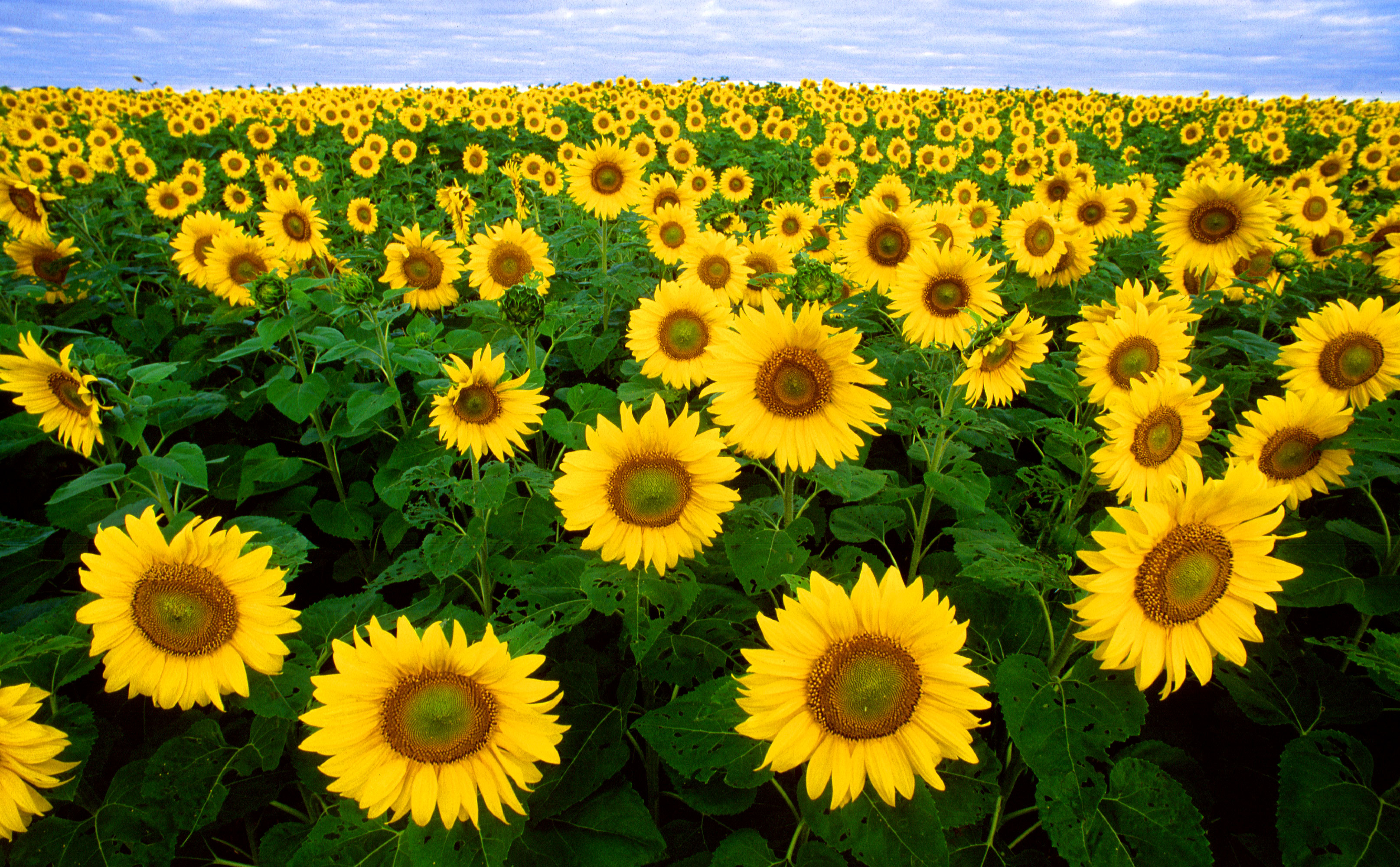
Fig. 7.1 Sunflowers. The size (scale) of the objects is dependent on the distance from the camera. A visual system should be prepared to ‘see’ objects at all possible sizes.
The image in Fig. 7.1 is a nice illustration of this effect. The flowers in the front are easily 10 times larger then the flowers near the horizon. Instead of flowers we could equally well look at faces at different distances (and thus size) or at license plates of cars at different distances from the camera.
The only sensible thing to do then is to be prepared for all possible sizes. The image should be processed at all levels of scales simultaneously. In a previous chapter we have already discussed the local structure of images and described that the scale of local details is characterized with the scale of the Gaussian smoothing kernel with which the image is smoothed.
Processing an image at all \(s>0\) leads to what is called a scale-space.
In this chapter we look at linear scale-space that is made by convolving a zero-scale image with Gaussian kernels of all sizes \(s>0\). We will discuss the definition and properties. When convolving an image with a Gaussian kernel we loose details is the image. Therefore the sampling distance can be enlarged resulting in less pixels and thus more efficient processing. This progressive smoothing and subsampling of images leads to image pyramics. Furthermore we look at one example of the use of a scale space, namely blob detection and localization in scale space.