(Laplacian) Scale Space

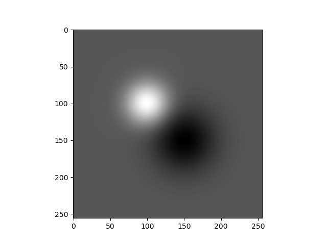
Two Gaussian Blobs.

The crux of the scale invariant feature transform is that Gaussian blobs in an image show up as extreme in the scale normalized Laplacian scale space \(\ell(\v x,s)\) (see the section on Linear Scale Space):

\[\ell(\v x, s) = s^2 (f \ast (G^s_{xx} + G^s_{yy}))(\v x)\]

If we have an image with a Gaussian blob of scale \(s_b\) at position \(\v x_0\) it is not hard to prove that we find an extremum in \(\ell(\v x, s)\) at \(\v x=\v x_0\) and \(s=s_b\). This is true for an isolated blob. For blobs closer together or images that show blob like structures it remains true that we find extrema in the Laplacian scale space at the scale of the blob and at its position in space.

Note that at large enough scale (i.e. after convolving with large scale Gaussian filters) almost everything in an image will start to look like Gaussian blobs.

Below we give the proof (click on the bar to show the proof) for an isolated blob. Even for that simple case the proof is not difficult but quite lengthy and so we use Mathematica…).

Proof (Blob in Scale-Space)

We define the image \(f\) showing a blob at position \((0,0)\) with scale \(s_b\) as the Gaussian function

\[f(x, y) = G^{s_b}(x, y) = \frac{1}{s_b\sqrt{2\pi}} e^{-\frac{x^2+y^2}{2s_b^2}}\]

In the Laplacian scale space we get

\[\begin{split}\ell(x, y, s) &= s^2\left( \pfrac{^2G^\sqrt{s^2+s_b^2}(x,y)}{x^2} + \pfrac{^2G^\sqrt{s^2+s_b^2}(x,y)}{y^2} \right)\\ &= s^2\left( G^\sqrt{s^2+s_b^2}_{xx}(x,y) + G^\sqrt{s^2+s_b^2}_{yy}(x,y) \right)\end{split}\]

The extrema in \(\ell(x,y,s)\) are found by solving the equations \(\ell_x(x,y,s)=0\), \(\ell_y(x,y,s)=0\) and \(\ell_s(x,y,s)=0\) for \(x\), \(y\) and \(s\).

This is a typical proof that I like to use a symbolic math program for. Below you find the Mathematica notebook for this:

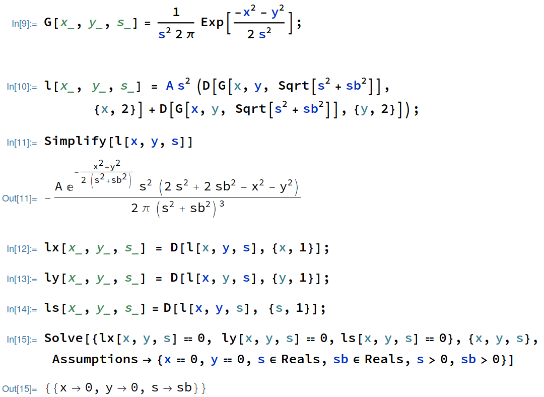
Yes indeed we have cheated a little here as we have assumed that the extremum is at \(x=0\), \(y=0\). Only assuming that \(x\) and \(y\) are real values we not only get the extremum at the origin but also a continuum of saddle points (see the Mathematical Tools part chapter on least squares estimators), i.e. points where all three derivatives are equal zero but the eigenvalues of the Hessian matrix are of mixed sign.

Calculating Scale-Space

Given the Gaussian derivative convolution encoded in the Python function gD

A linear scale space is nothing else than a stack of images that blurred with increasingly larger Gaussian kernels. Let \(f^{s_0}\) be the starting image whose scale is assumed to be \(s_0\) (where it is often assumed that \(s_0=0.5\)). From this image we then build the scale space:

\[f(\v x, s) = (f^{s_0} \ast G^{\sqrt{s^2-s_0^2}})(\v x)\]

Because Gaussian smoothing commutes with calculating the derivative (any derivative) we have

\[\partial_{..} f(\v x, s) = (\partial_{..} f^{s_0} \ast G^\sqrt{s^2-s_0^2})(\v x)\]

where \(\partial_{..}\) stands for any spatial derivative. Evidently, as seen before, the more sensible way to implement this is:

\[\partial_{..} f(\v x, s) = (f^{s_0} \ast \partial_{..} G^\sqrt{s^2-s_0^2})(\v x)\]

Scale should be sampled logarithmically, i.e. an equidistant sampling in the \(\log(s)\) parameter.

\[s_i = s_0 \alpha^i\]

and thus:

\[\begin{split}f(\v x, s_i) &= (f^{s_0} \ast G^\sqrt{s_i^2-s_0^2})(\v x) \\ &= (f^{s_0} \ast G^\sqrt{s_0^2\; \alpha^{2i}-s_0^2})(\v x) \\ &= (f^{s_0} \ast G^{s_0 \sqrt{ \alpha^{2i}-1}})(\v x) \\\end{split}\]

In the scale invariant feature transform SIFT the keypoint are found as the extrema in the scale normalized Laplacian scale space:

\[\ell(\v x, s) = s^2 (f \ast (G^s_{xx} + G^s_{yy}))(\v x)\]

This idea was pionered (and invented?) by Toni Lindenberg. It is easy to calculate that in case an image contains a Gaussian blob at scale \(s_b\) there is an extremum in the Laplacian scale space at the center of the blob and at scale \(s_b\). All blobs when smoothed with a Gaussian kernel are ‘lookin like’ Gaussian blobs and thus extrema in the Laplacian scale space are points that we may hope for to find in images in a translation, rotationally and scale invariant way.

Finding the extrema is discussed in a subsequent section. When we also want to find the extrema at subpixel accuracy we need to calculate the first and second order derivatives of \(\ell\) both spatial as well as scale derivatives. These corresponds with derivatives of \(f\) up to order four.

The original implementation of the SIFT algorithm approximates the Laplacian scale space as a difference of Gaussians (DoG) stack. Let \(f\) be the Gaussian (zero order) scale space then it is not hard to prove that

\[\ell(\v x, s) \approx \frac{1}{\alpha - 1}\left( f(\v x, \alpha s) - f(\v x, s)\right)\]

Proof:

We start with the difference in first order approximation

\[\begin{split}f(\v x, \alpha s) - f(\v x, s) &= f(\v x, s) + (\alpha -1) s f_s(\v x, s) - f(\v x, s)\\ &= (\alpha - 1) s f_s(\v x, s) \\ &= (\alpha - 1) s^2 (f_{xx}(\v x, s) + f_{yy}(\v x, s))\end{split}\]

and thus

\[\ell(\v x, s) = s^2 (f_{xx}(\v x, s) + f_{yy}(\v x, s)) = \frac{1}{\alpha - 1}\left(f(\v x, \alpha s) - f(\v x, s)\right)\]

Here we deviate from the Lowe (and OpenCV) implementation. In our simplest implementation we will generate the ‘real’ Laplacian scale space (instead of the difference of Gaussians scale space). In the second implementation we won’t use finite differences for the subpixel extrema localization and replace them with Gaussian derivatives as well. Then we need Gaussian derivatives up to order four.

Calculating the Laplacian Scale Space

All we have to do is calculate \(\ell(\v x, s)\) for several values of \(s\). We assume the original image is observed at scale \(s_0\) and thus

\[\ell(\v x, s_i) = s^2 \left( f^{s_0} \ast G_{xx}^{s_0\sqrt{\alpha^{2i}-1}} + f^{s_0} \ast G_{yy}^{s_0\sqrt{\alpha^{2i}-1}} \right)\]

In accordance with Lowe we select a value of \(\alpha\) such that \(s_0 \alpha^K = 2\) where the images in the range from \(s\) to \(2s\) is called an octave (don’t be confused: there is no number 8 involved, the octave refers to the tone interval where frequency is doubled).

For illustration assume \(K=4\) then the first octave is:

\[s_0 = \alpha^0 s_0 \quad \alpha^1 s_0\quad \alpha^2 s_0\quad \alpha^3 s_0\quad \alpha^4 s_0=2 s_0\]

The second octave then starts at \(2 s_0\) and ends at \(4 s_0\), etc. For a total of \(L\) octaves.

All images are in the same resolution of the original image and are stored in an array of shape (KL+1, M, N) where (M,N) is the shape of the original image.

We assume the gD function is available to calculate the Gaussian derivative function.

K = 4 # number of scales in octave
L = 5 % number of octaves
scales = np.logscale(0,L,num=K, endpoint=True)
print(scales)

def make_laplacian_scale_space(f, scales):
    f = zeros((len(scales), *f.shape))
    for l, s in enumerate(scales):
        f[l, :, :] = gD(f, s, (2,0)) + gD(f, s, (0,2))

Calculating the 4-jet

The 4-jet is the collection of image derivatives up to order 4 for all scales

\begin{gather} f\\ f_x\quad f_y \\ f_{xx} \quad f_{xy} \quad f_{yy} \\ f_{xxx} \quad f_{xxy} \quad f_{xyy} \quad f_{yyy} \\ f_{xxxx} \quad f_{xxxy} \quad f_{xxyy} \quad f_{xyyy} \quad f_{yyyy} \\ \end{gather}