Scale Invariant Feature Transform
Consider the task of recognizing corresponding points in two images of the same object.
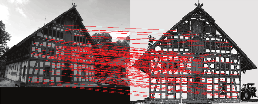
SIFT. Finding characteristic points in images irrespective of scale, translation, rotation and affine gray scale changes.
Note that a/ the left image is much darker than the right image, b/ the scale of the two images is (slightly) different, the orientation—due to slightly different angle of the camera with respect to the front of the house—is slightly different. Still the SIFT algorithm is capable of finding the characteristic points in both images, together with a point descriptor that allows us to compare a point in the left image and a point in the right image and decide whether they probably correspond with the same 3D scene point.
Perhaps the most often cited article in Computer Vision before 2012 1 is “Object Recognition from Local Scale-Invariant Features”. It has been cited over 20000 times. It was the first system that was capable of doing this in a robust way.
The SIFT paper is really a hard paper to read, especially if it is your goal to implement the algorithm yourself. In this chapter we walk you through understanding the Scale Invariant Feature Transform (SIFT).
The classical SIFT algorithm aims at:
defining points in an image that are invariant under translation, rotation, scale and affine grey scale changes.
describing these points in such a way that points in different images can be compared. Again with all invariances as given above.
These points, together with their descriptor, are called the key points. The result of the SIFT algorithm is a list of tuples of the form \((\v x, s, \theta, \v d)\) where
\(\v x\): a key point location (\(x\) and \(y\) coordinates)
\(s\): the scale at which the key point is found
\(\theta\): the orientation of the key point
\(\v d\): the descriptor that describes the appearance of the neighborhood of the point \(\v x\).
The basic steps in the classical SIFT algorithm are:
Building the Laplacian scale space
Detecting the extrema in the Laplacian scale space on a course grid in scale space (space times scale).
Subpixel localization of these extrema. The first three steps result in a list of key point tuples \((\v x, s)\).
Calculating the orientation per key point resulting in a list of tuples \((\v x, s, \theta)\).
Calculating a descriptor for each key point that describes its neighborhood resulting in the final list of tuples \((\v x, s, \theta, \v d)\).
In this chapter we will describe these steps in separate sections.
Footnotes
- 1
In 2012 the paper on AlexNet was published describing the CNN that outperformed all traditional methods to classify the objects visible in images. That article is now referenced more than 100000 times.