5.2.12. Active Analog Filters

In a previous section we already have shown a low pass filter build from passive components. We repeat the passive circuit below.

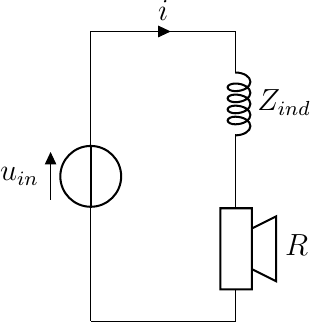
The advantage of such a passive speaker is that it can handle a lot of power (100-200 Watt speaker drivers are not uncommon). A disadvantage is that the speaker parameters (the speaker impedance in this case) are important in the transfer function. Also passive elements that are capable of handling a lot of power are expensive.

In the design of active filters most often capacitors are used, so let’s first show a passive filter using a capacitor. First we show the filter without the load.

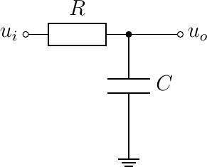
This is a simple voltage divider but with a complex impedance \(Z_\text{capacitor}=1/(j\w C)\). We thus have

\[\begin{split}u_o &= \frac{Z_c}{R+Z_c} u_i\\ &= \frac{\frac{1}{j\w C}}{R+\frac{1}{j\w C}} u_i\\ &= \frac{1}{1+j\w RC} u_i\end{split}\]

That is the frequency response of this filter is:

\[H(\w) = \frac{1}{1+j\w RC}\]

and plotted in the figure below.

Show code for figure

import numpy as np
import matplotlib.pyplot as plt

plt.clf()
w = np.logspace(-3, 2)
Hw = 1 / (1 + 1j * w)
fig, (axreal, aximag) = plt.subplots(nrows=2, sharex=True);
axreal.plot(w, np.abs(Hw) );
axreal.set_xscale('log')
axreal.set_yscale('log')
axreal.set_xlabel('$\omega$');
axreal.set_ylabel(r'$|H(\omega)|$');

aximag.plot(w, np.angle(Hw));
aximag.set_xscale('log')
aximag.set_xlabel('$\omega$');
aximag.set_ylabel(r'$\angle H(\omega)$');
plt.savefig('source/figures/lowpassfreqresp.png')

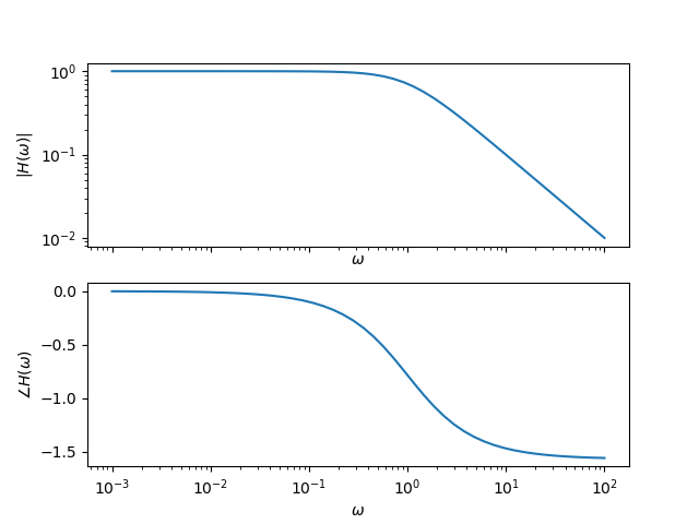
Fig. 5.23 Frequency response of a low pass filter. Plotted are the absolute value (magnitude) and phase (angle) part of the function \(H(\w)\) (with \(R=C=1\)).

Comparing this with the low-pass filter from a previous section we see that this is indeed the transfer function of a low-pass filter but know with cut-off frequency \(\w_c = 1/(RC)\). But in case we would have low impedance speaker at the output (speakers are most often in the range from 4 to 16 Ohm’s) the speaker impedance will greatly influence the transfer function. A simple unity gain opamp circuit (with a very high input impedance) will act as a buffer and will make the transferfunction independent of the load (i.e. the circuit at the output).

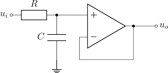
For the circuit above we still have that \(u_o=u_i\) but for this circuit this is (almost) independent of the load. The unity gain amplifier in the circuit above can be replaced with a non-inverting amplifier as sketched in the figure below.

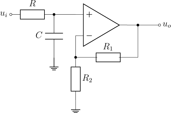
Fig. 5.24 Low pass filter with amplification.

The frequency response of this filter is

\[H(\w) = \left(1+\frac{R_1}{R_2}\right)\frac{1}{1+j\w RC}\]

The proof is left as an exercise for the reader in this chapter.

Finally we give an OpAmp circuit that is used a lot in analog signal processing: the Sallen-Key topology.

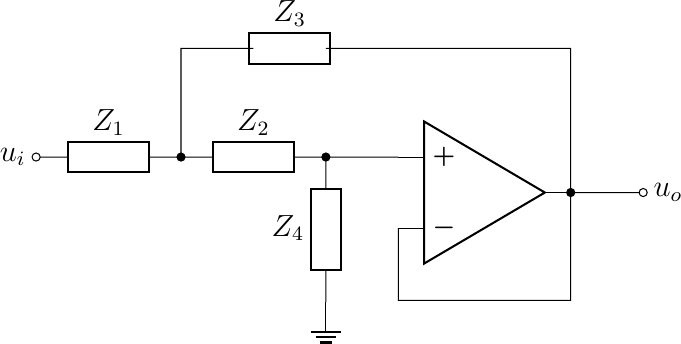
Fig. 5.25 Sallen-Key Generic Filter.

The transfer function for this filter is:

\[\frac{u_o}{u_i} = \frac{Z_3 Z_4}{ Z_1 Z_2 + Z_3(Z_1 + Z_2) + Z_3 Z_4}\]

Depending on the types of impedance (complex or not) different frequency responses can be realized. A second order unity gain high-pass filter can be realized with the filter shown below.

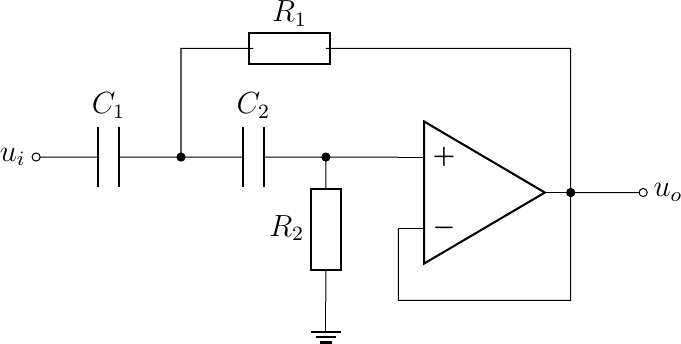
Fig. 5.26 Sallen-Key Unity-Gain High-Pass Filter.

The resulting filter is a second order high-pass filter. The frequency response of such a filter is determined by two parameters, its cut-off frequency and its \(Q\)-factor (see the chapter on filters). From the figure of the filter circuit it’s clear that we have 4 parameters (2 capacitances and 2 resistances). The choice for the values of this redundant set of parameters (redundant as far as its frequency response is concerned) is up to electrical engineers (see Wikipedia or the book The Art of Electronics by Horowitz and Hill, the bible for classic electronic engineers).

The transfer function of the unity gain high pass filter in the s-domain (see the chapter on the s-domain):

\[H(s) = \frac{s^2}{s^2 + \frac{\w_0}{Q} s + \w_0^2}\]

where

\[\begin{split}\w_0 &= \frac{1}{\sqrt{R_1 R_2 C_1 C_2}}\\ Q &= \frac{\sqrt{R_1 R_2 C_1 C_2}}{R_1(C_1+C_2)}\end{split}\]