1.4. Exercises
Write Python functions to plot signals/functions. You should be able to plot real as well as complex signals and CT as well as DT signals. You will be using this functionality quite a lot in this course.
Plot the following functions:
Step functions \(u(t)\) and \(u[n]\).
Translated stepfunctions \(u(t-2)\) and \(u[n-2]\)
Scaled and translated step function \(3\, u(\frac{t-2}{3})\)
Plot the \(x_a\) function for several values of \(a\). See for yourself that it starts to look as the pulse function.
Defining the CT pulse function as the limit of the \(x_a\) function is not a unique definition. If we take the function \(g_s(t)\) being the Gaussian function (you may well remember…) and look at the limit for \(s\rightarrow0\) you will see that in the limit we arrive at the pulse function too. Plot the \(g_s\) for several values of \(s\) to see for yourself.
Consider the CT complex exponential functions
\[\begin{split}x(t) &= e^{j 3\pi t / 4}\\ x[n] &= e^{j 3\pi n / 4}\end{split}\]Show code for figure
 1import numpy as np
 2import matplotlib.pyplot as plt
 3
 4plt.clf()
 5t = np.linspace(0, 15, 1000)
 6n = np.arange(16)
 7xct = np.exp(1j*3*np.pi*t/4)
 8xdt = np.exp(1j*3*np.pi*n/4)
 9plt.subplot(2,1,1)
10plt.plot(t, xct.imag)
11plt.subplot(2,1,2)
12plt.stem(n, xdt.imag, use_line_collection=True)
13plt.savefig('source/figures/complexexponentialexample.png')
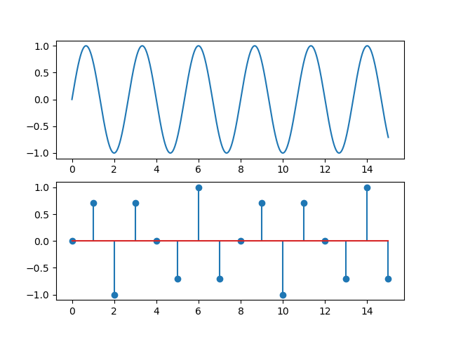
Fig. 1.12 Complex exponential \(e^{j 3\pi t / 4}\) (top) and \(e^{j 3\pi n / 4}\) (bottom).
what is the period of \(x(t)\)?
what is the period of \(x[n]\)?