5.5.4. Control Systems

5.5.4.1. Feedback Control System

Consider a system where we heat the water in a tank. We set a temperature, say 70 degrees. We compare the set temperature (set value) with the actual temperature (the process value). The error is used to control the heater. In case the set value minus the process value is positive we need to heat the water, in case the difference (error) is negative we should cool the water.

In a process diagram this leads to a block diagram like:

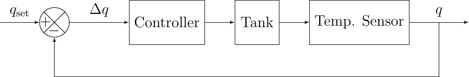
Fig. 5.56 A Heated Water Tank

We assume that all blocks in such a scheme represent linear time invariant systems. In that case each system can be represented with its transfer function \(H_i(s)\). Representing all blocks in the \(s\) domain we get:

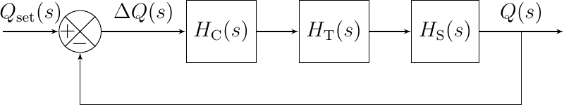
Fig. 5.57 A Heated Water Tank (s-domain)

This system is equivalent with a unit feedback system with open loop transfer function:

\[H_1(s) = H_{\text{C}}(s)\; H_{\text{T}}(s)\; H_{\text{S}}(s)\]

and total transfer function:

\[H(s) = \frac{H_{\text{C}}(s)\; H_{\text{T}}(s)\; H_{\text{S}}(s)}{ 1 + H_{\text{C}}(s)\; H_{\text{T}}(s)\; H_{\text{S}}(s)}\]

In simple control systems the task of the controller is to make sure that the error, difference between process value and set value remains zero. And in case it deviates from zero (due to a new value of the set value or an external disturbance) the system should recover in a stable and fast manner to arrive at an error zero again.

For the water tank system you could think of the situation that the set temperature at time \(t=0\) is changed from 50 degrees to 70 degrees. Or we might have the situation that the tank is filled with cold water, thus lowering the process value from 50 degrees to 40 degrees while the set temperature is still set at 50 degrees.

In both cases the system has to adapt to the new situation as fast as possible in a stable way.

5.5.4.2. Stability

Not all systems are stable systems. Think of balancing a broom stick on the top of your finger. Or walking on top of big ball. Or keeping a quadcopter in an upright position in the air.

Linear systems described with a transfer function \(H(s) = \frac{N(s)}{D(s)}\) are characterized by the zeros (zeros of \(N(s)\)) and poles (zeros of \(D(s)\)). We have that the system is:

• Stable: all poles left of the imaginairy axis,

• Marginally stable: poles left and on the imaginary axis

• Unstable: at least one pole on the right hand side of the imaginary axis.

Marginally stable systems tend to oscillate.

5.5.4.3. PID Controller

Consider the system \(H(s)\) (often called the plant in control theory) for which we are designing a (negative) feedback controller \(G(s)\).

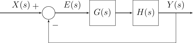
Fig. 5.58 Feedback Control

We start with the canonical first order system to be controlled:

\[H(s) = \frac{1}{\tau s + 1}\]

The root of this system is at \(s=-1/\tau\) and for any \(\tau>0\) this is a stable system. Nevertheless the need may arise to control this system to get a faster response. Most often the system cannot be changed to have a smaller time constant \(\tau\).

Let’s start with the simplest of all controllers: we only amplify the error signal, i.e.

\[G(s) = K_p\]

where the \(p\) stands for proportional. The total transfer function of the feedback system then is:

\[H_c(s) = \frac{K_p H(s)}{1 + K_p H(s)} = \frac{K_p}{\tau s + 1 + K_p}\]

where \(H_c\) is the transfer function of the controlled system. Now the pole of the controlled system is at \(s=-(1+K_p)/\tau\). Observe that for \(K_p>-1\) we still have a stable system. Evidently for \(K_p=0\) the system is ‘dead’ giving zero for every input.

Plotting the step response of the controlled system for some values of \(K_p>0\) we see that with larger \(K_p\) the system indeed responds faster but that the output does not asymptotically approach the (often) desired same asymptotic value as the uncontrolled system approaches (one is this case).

Show code for figure

import numpy as np
import matplotlib.pyplot as plt
from scipy import signal
import control as ctr

plt.clf()

tau = 1

t = np.linspace(0, 10, 1000)

H = ctr.tf([1], [tau, 1])
_, ystep = ctr.step_response(H, t)
plt.plot(t, ystep, '--', label=r'uncontrolled system ($\tau={}$)'.format(tau));


for Kp in [0, 1, 2, 3, 5, 9]:
    Hc = ctr.feedback(ctr.series(ctr.tf([Kp],[1]), H))
    _, ystep = ctr.step_response(Hc, t)
    plt.plot(t, ystep, label=r'controlled system ($K_p={}, \tau={}$)'.format(Kp, tau));


plt.legend();


plt.savefig('source/figures/controlledP1storder.png')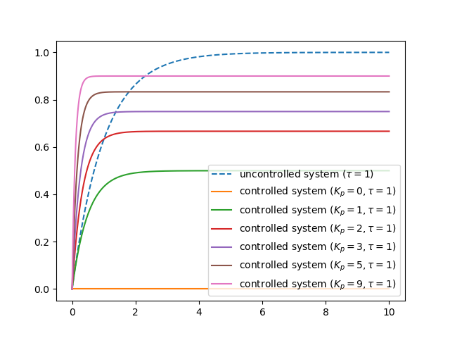

Fig. 5.59 Step Response of Controlled First Order System. The controller is a simple proportional controller with different values for \(K_p\). Also shown is the step response of the uncontrolled system.

From the figure above it is clear that the response becomes faster indeed but that the stable value (for large \(t\)) is smaller than one. We could correct with a gain block in series with the entire controlled system.

A better way to compensate for the asymptotic error is to incorporate a parallel path with an integrator in the controller.

\[G(s) = K_p + \frac{K_i}{s}\]

We set \(K_p\) equal to two and consider different values for \(K_i\).

Show code for figure

import numpy as np
import matplotlib.pyplot as plt
from scipy import signal
import control as ctr

plt.clf()

tau = 1
Kp = 2

t = np.linspace(0, 10, 1000)

H = ctr.tf([1], [tau, 1])
_, ystep = ctr.step_response(H, t)
plt.plot(t, ystep, '--', label=r'uncontrolled system ($\tau={}$)'.format(tau));


for Ki in [0, 1, 2, 3, 5, 9]:
    Hc = ctr.feedback(ctr.series(ctr.parallel(ctr.tf([Kp],[1]), ctr.tf([Ki], [1, 0])), H))
    _, ystep = ctr.step_response(Hc, t)
    plt.plot(t, ystep, label=r'$K_i = {}, K_p={}, \tau={}$)'.format(Ki, Kp, tau));


plt.legend();


plt.savefig('source/figures/controlledPI1storder.png')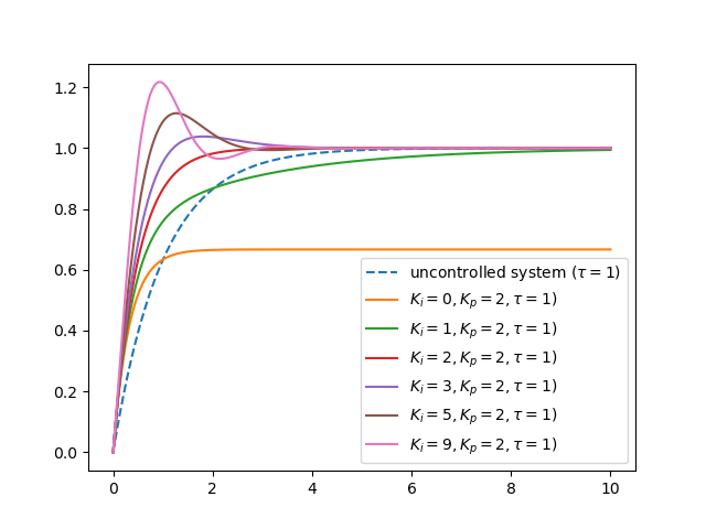

Fig. 5.60 Step Response of Controlled First Order System. The controller is a proportional controller in parallel with an integrating controller. Also shown is the step response of the uncontrolled system.

Note that adding a integral controller to the mix makes the total system into a second order system. The advantage as can be seen in the figure is that the response can be faster and with \(K_i>0\) the asymptotic error will vanish. A disadvantage is that we can introduce overshoot in the response as can be clearly seen in the figure.

There is a third type of often used controller: the derivative controller. The total control system then becomes:

\[G(s) = K_p + K_i \frac{1}{s} + K_d s\]

Such a controller is called a PID controller consisting of three parallel subsystems: Proportional (gain), Integrate and Derivative.

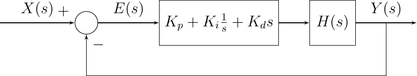
Fig. 5.61 PID Control

In such a generic PID controller we need to select the three constants \(K_p\), \(K_i\) and \(K_d\) to achieve the goal of the controller. The classical way of doing so is to first reduce the problem to a one parameter problem, either by fixing two of the three parameters or by setting \(K=K_p\), \(K_i=\alpha K\) and \(K_d = \beta K\) where \(\alpha\) and \(\beta\) are selected constants. In that case the influence of the factor \(K\) can be analyzed using root locus analysis.

To select all parameters there are also some heuristic PID design methods of which the Ziegler-Nichols tuning is a famous one.

And in practice some of the Ziegler-Nichols tuning method is used: namely to first start with \(K_i=K_d=0\) and then selecting the \(K_p\) such that a stable oscillation is obtained. Then the other parameters are selected by simply trial and error.

In this section we only considered a simple example of a PI controller to decrease the tine in which a system reaches it steady state. A far more important use of PID controllers to take an initial system \(H(s)\) that is unstable and through the use of an appropriate PID control make it into a stable system. For such use the root locus analysis method is of great help.

5.5.4.4. Root Locus Analysis