5.1. Sound and Sound Processing
5.1.1. What is sound?
The human ear measures time dependent air pressure and transforms these pressure variations into electrical signals that are fed into our brain and give us the sensation of what we call sound.
A sound source (a human voice, a piano, a hand hitting the table, etc) causes pressure changes in the air. These pressure differences propagate in the air giving rise to a sound wave.
When you throw a pebble in water you see a wave propagating outwards in concentric circles. The displacement of the water in the wave is perpendicular to the direction in which the wave travels: the wave moves horizontally, the water itself moves up and down. Water waves are transverse waves.
On the other when you hit the table with your hand the sound wave eminating from that point is a longitudinal wave: the air moves forward and backward in the direction in which the wave also moves.
Fig. 5.1 Airpressure Wave, traveling from loudspeaker to ear.
In the figure above the loudspeaker on the left vibrates and causes the air to vibrate with it (from http://www.mediacollege.com) . The air molecules close to the speaker are forced away from the speaker, colliding into the next ‘layer’ of molecules. These molecules start vibrating as well and collide into the next layer etc. In this way the vibration is transported through the air. Note that the air particles do not travel from left to right. (see the page http://www.acs.psu.edu/drussell/demos.html with some very nice animations and explanations).
The dots in the figure illustrate where there are many molecules per unit volume (i.e. high pressure) and where there are less (low pressure). This variation in pressure, at one moment in time, can be characterized as a function of pressure agains position from speaker to ear (the lower plot).
If we would make a movie of the wave propagation we would see the layers of high pressure (compression) and low pressure (rarefaction) travel from left to right.
Fig. 5.2 Longitudal wave, travelling from left to right in space. This time the density of the air particles is depicted with lines. The closer lines are to eachother the higher the pressure. We see one high pressure vertically elongated area going from left to right.
In the figure above the differences in the air pressure are illustrated as the density of the grid lines (illlustration from Wikipedia).
See http://www.acoustics.salford.ac.uk/feschools/index.htm for a nice intro to acoustic waves and some nice animations.
In case we measure the (sound) pressure in one point in place as a function of time we obtain a function \(f(t)\). Note that the function depends very much on the position in space where you measure the sound pressure.
5.1.2. Human Perception of Sound
The pressure differences travelling through the air ‘hit’ the tympanic membrane in the outer ear (the eardrum). Through an intricate mechanical system of small bones this vibration is transported (and amplified) to another membrane: the oval window. The oval window is the membrane that is at the start of the cochlea, a rolled-up space of two compartments separated by the basilar membrane filled with fluid.
Fig. 5.3 The human ear, both external as well as internal.
The vibrating membrane at the oval window makes the fluid particles vibrate. The shape of the cochlea and the membrane is such that high frequenties in the sound make the hair cells at the base of the basilar membrane respond, lower frequencies in the sound make hair cells at the end of the basilar membrane respond.
Fig. 5.4 The Cochlea, the human sound sensor.
The human hearing system thus not sample the audio (pressure) signal but it does a real time “Fourier” analysis of the sound signal and samples the frequency components. For a lot of computer audio processing this first step in audio analysis is mimiced.
The responses of the hair cells are transmitted to the brain where they are perceived. The hearing brain does not record audio signals as we do when sampling and storing a sound signal. In sound perception a lot of sound analysis is done as well. So computer scientists cannot do a lot of usefull computer audio processing without knowing the basics of psychoacoustics.
5.1.2.1. High Frequency Limit
The ‘average’ human ear can hear sounds in the range from 20Hz to 20,000 Hz. Combined with the sampling theorem of Shannon-Nyquist it follows that sound can be sampled at around 40,000 Hz. I.e. if the goal is to reproduce the sound for a human ear. And of course we should make sure that the signal that is sampled indeed does not contain components at frequency higher than half the sample frequency. This is often done using a analog low pass filter when recording analog sound signals. When subsampling discrete signals a discrete low pass filter can be used (see later section).
5.1.2.2. Absolute Threshold of Hearing
Not all frequencies are perceived equally load. In fact the sound pressure level that is needed to hear sounds at equal loudness (a subjective measure) depends on the frequency of the sound. The sound pressure as a function of frequency of a just noticible sound is called the absolute threshold of hearing (ATH). This function is depicted in the figure below.

Fig. 5.5 Absolute Threshold of Hearing.
From this figure we may observe:
lower frequency sounds need relatively more power to be heard,
frequencies in the range of about 2000-4000 Hz are best heard by the human ear (these are important frequencies for voice recognition), and
for higher frequencies more power is needed again.
The ATH is just one equal loudness contour. For higher loudness the corresponding contours are more or less vertically shifted versions as can be seen in the figure below:
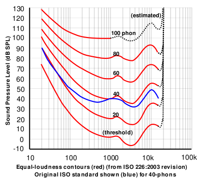
Fig. 5.6 Equal Loudness Contours.
The lowest red function is the ATH curve.
5.1.2.3. Simultaneous Masking
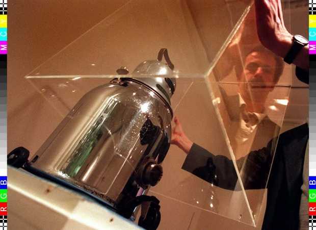
The Dutch writer Simon Vestdijk used to turn on his vacuum cleaner
in order not to be disturbed by other sounds when writing (yes the
vacuum cleaner is really on exhibit in a Dutch museum, see the
picture). When you listen to a vacuum cleaner you realize that the sound is very
much like white noise.
White noise is a sound that contains all audible frequencies. It is really noise: you can make white noise by generating random values for each sample in the sound signal.
Because white noise contains all frequencies it masks all frequencies as well. So Vestdijk’s vacuum cleaner was a cleverly chosen household appliance to make the noise not to distract him from his work.
If we make noise with less high frequencies we obtain
brown noise (not to be confused
with the myth of the brown note: see Mythbusters and
Southpark). Brown noise is used in recordings that alledgedly help
you in having an undisturbed powernap. There are even chrome extensions that play
these noise sounds to keep you focussed (refresh the page that is
linked to until you get a real noise like sound).
Vestdijk was way ahead of his time! And this trick surely kept him focussed. He is known as the author who “wrote faster than God could read”.
Simultaneous masking refers to the phenomenon where a sound with say frequency masks a sound with a frequency close to it. This effect can be modelled as a change in the ATH curve.
In the above figure the ATH is changed due to a dominant sound at frequency of 1KHz. The masking effect is such that other sounds in the range from say 0.5 to 5 KHz need a higher sound pressure level to be heard compared with the sound level as dictated by the ATH curve.
5.1.2.4. Temporal Masking
Besides simultaneous masking the human ear masks sounds that occur not only simulaneously but also sound are masked that occur later (post-masking). That seems plausible, just after you have heard a loud sound you cannot hear other sounds that are of lower volume. Your auditory system more or less needs to unwind to hear the softer sounds again.
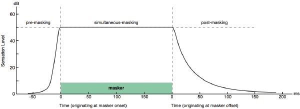
There is also a pre-masking effect: you do not hear a low volume sound just before a louder masking sound is heard. The pre-masking effect seems to defy causality (how can an effect occur before the cause?). In fact it doesn’t: like any other nervous system the auditory systems exhibits a latency. It that deferred processing and awareness that makes that although the low volume sound is ‘recorded’ earlier then the masking sound (it couldn’t be otherwise) it is processed (and suppressed) when the louder signal came in just somewhat later.
5.1.3. Sound Level Measurement
In a lot of the figures in this section the sound level was given in dB, short for decibel. This is a logarithmic scale that indicates the ratio between two audio power levels:
In case we consider the amplitudes of sound signals:
due to the fact that the power is proportional to the square of the amplitudes.
Despite the fact that audio levels are expressed most often in decibels (dB) and thus must involve two levels you most often see it used to indicate the strength of just one audio signal. Implicitly then most often the power level that corresponds with just noticible sound is used as the second power level (\(P_2\) or \(A_2\) in the above formules).
In the table below several sounds and the associated sound pressure level (in dB) are given (from Wikipedia):
Sound |
AirSound Pressure Level (dB) |
|---|---|
Jet engine at 30 m |
150 |
Threshold of pain |
130 |
Vuvuzela at 1 m |
120 |
Hearing damage |
120 |
Jet engine at 100 m |
110-140 |
Busy traffic at 10 m |
80-90 |
Hearing damage (long term exposure) |
85 |
Passenger car at 10 m |
60-80 |
TV at 1 m |
60 |
Dishwasher |
42-53 |
Normal conversation |
40-60 |
Very calm room |
20-30 |
Auditory threshold (at 1 kHz) |
0 |
5.1.4. A word of warning
Nowadays the sound level at (pop) concerts is very high (100+ dB). The Dutch ARBO law (protecting people against working condition hazards) states that people are allowed to work for at most 5 minutes in an environment with a 100 dB sound level without protection (have you noticed that most people working at the concert you are visiting do wear protective earplugs…)
Please read: http://nl.wikipedia.org/wiki/Lawaaidoofheid and take precautions.
5.1.5. Sound Recording
Sound is recorded using a microphone: a device that transforms the pressure variations in a medium into an electronic signal. This analog signal is discritized by quantization and sampling.
The quantization for human audible sound is most often done using 16 bits AD convertors. For these convertors every step in the quantization scheme corresponds with an equal interval of the sound amplitude.
The number of samples per second for music is most often set at 44000 Hz. This value is about twice the highest frequency that can be heard by the human ear. Be aware that the recording device needs to filter the frequencies higher then half the sample frequency such that aliasing artefacts cannot occur.
If you are not recording polyphonic music but ‘only’ in speech recording (and transmission) the sample frequency can be chosen much lower at about 8000 Hz implying the for speech we need frequencies up to 4KHz to be faithfully reproduced.
5.1.6. Sound Compression
Sampling a stereo sound signal at 44100 Hz with a 16 bit quantization for each of the channels leads to around 635 MByte per hour of music. That is about the storage capacity of an ‘old fashioned’ CD. Indeed that was the goal at Philips Research Labs: make a digital version of long play record that was capable of storing about an hour music (using both sides…).
Nowadays we are used to mp3, aac, ogg and other sound compression methods that are able to compress the music considerably without too much loss of audio quality. But there is inevitably some loss involved.
Lossless data compression algorithms do exist for sound (like flac) but the compression ratio is most often below 2 (i.e. the compressed file then is about half the size of the original file) when used for music.
This is a far lower compression ratio then we are used to when using one of the mentioned compression schemes. These schemes are capable of better compression ratios using a lossy compression technique, ‘throwing away’ only that information in the sound that cannot be heard by the human listenes.
Most lossy sound compression techniques are based on our limitations of hearing. The frequency dependence of our ability to hear sounds (captured in the equal sound level curves), the masking effects (both simultaneous and temporal), all these are used in compression to reduce the number of bits that are needed to represent the sound signal. Perceptual coders are among the best performing audio (and video) coders.
Compression of speech as used for instance in GSM mobile phones and in the speech encoding for video conferencing is based on a model for speech generation. A crude model of what the vocal tract does with the basic sound (a simple buzz) is used. The parameters of this model are dependent on what is actually heard. These parameters are estimated from a short time interval in the sound and instead of coding the sound signal itself, the model parameters need to be transmitted (or stored). The decoder then can reconstruct the sound (well not quite.. but at least we hear the same utterance).