2.2. Convolutions

The main result and take away message from this section is that any LTI system is a convolution and is completely determined by its impulse response function.

In the first subsection we derive that equivalence for both CT and DT systems. In the second subsection we give a recap of what a convolution actually does and state some of its properties.

2.2.1. Linearity + Translation Invariance = Convolution

A linear shift invariant system can be described as a convolution of the input signal. The kernel used in the convolution is the impulse response of the system.

Fig. 2.7 A CT Shift Invariant Linear System is characterized with its impulse response.

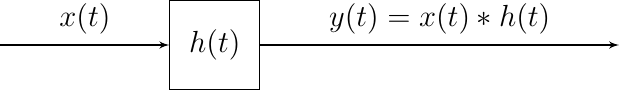
A proof for this fact is easiest for discrete time signals. That proof for discrete time signals is left as an exerise for the reader. Here we consider continuous time signals.

Let \(x\) be the input signal to a linear system \(\op L\) and let the output be \(y=\op L x\). We can write \(x\) as an integration (summation) of shifted pulses:

\[x(t) = \int_{-\infty}^{\infty} x(u)\delta(u-t)du\]

Because \(\delta(x)=\delta(-x)\) we can also write:

\[x(t) = \int_{-\infty}^{\infty} x(u)\delta(t-u)du = \int_{-\infty}^{\infty} x(u)\delta_u(t)du\]

where \(\delta_u(t)\) is the function \(\delta\) shifted to the left over \(u\). Now look at \(\op L x\). Because of the linearity of \(\op L\) we may write:

\[(\op L x)(t) = \int_{-\infty}^{\infty} x(u)(\op L\delta_u)(t)du\]

Shift invariance of the operator implies that \((\op L\delta_u)=(\op L \delta)_u\), i.e. first shifting and then applying the operator is the same as first applying the operator and then shift.

Obviously \(\op L \delta\) is the pulse response of the linear system, let’s call it the function \(h\), then we get:

\[(\op L x)(t) = y(t) = \int_{-\infty}^{\infty} x(u)h(t-u)du\]

or equivalently:

\[y = x \ast h\]

the output of a shift invariant system is given by the convolution of the input signal with the impulse response function of the system. In the signal processing literature it is common to write:

\[y(t) = x(t) \ast h(t)\]

Although this is a bit sloppy notation (for a mathematician this looks like an expression involving real numbers not functions) it is used a lot and even in some cases it helps to make clear what the functions involved are.

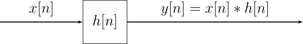
Consider the case of discrete time signals. Let \(x[n]\) be the input signal to a linear LTI system that is characterized with its impulse response \(h[n]\). The output signal then is given by:

\[y[n] = x[n] \ast h[n] = \sum_{k=-\infty}^{\infty} x[n-k]\; h[k]\]

So although mathematically quite sloppy, this notation allows for clear distinction between coninuous time and discrete time systems.

Fig. 2.8 A DT Shift Invariant Linear System is characterized with its impulse response.

2.2.2. Properties and Recipe

Definition 2.1 (Convolution)

A convolution of a signal \(x\) with a kernel (impulse response) \(h\) is defined as

CT	DT
\[\] x[n] ast h[n] = sum_{k=-infty}^{infty} x[n-k] h[b]	\[\] x(t) ast h(t) = int_{-infty}^{infty} x(t-u);h(u) du

Given a signal \(x\) and kernel \(h\) the recipe to calculate the convolution \(x\ast h\) is

Recipe for Convolution
CT		DT
\(h^\star(t)=h(-t)\)	1, Mirror the kernel	\(h^\star[n] = h[-n]\)
\(h^\star(t-u)\)	2. Shift the kernel to time \(u\) (sample k)	\(h^\star[n-k]\)
\(x(t)\;h^\star(t-u)\)	3. Multiply with the signal \(x\)	\(x[n]\;h^\star[n-k)\)
\((x\ast h)(u) = \int_{-\infty}^{\infty} x(t)\;h^\star(t-u) dt\)	Integrate (sum)	\((x\ast h)[k] = \sum_{n=-\infty}^{\infty} x[n]\;h^\star[n-k)\)

The above recipe in nicely illustrated in this webpage of which a screenshot is shown in the figure below.

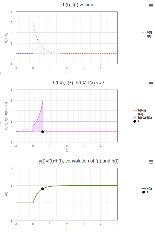
Fig. 2.9 Convolution of \(f\) and \(h\). The figure is a screenshot of an interactive illustration of the convolution recipe on this website .

Theorem 2.2 (Commutativity)

Convolution is commutative. Let \(x\) and \(y\) be two signals (both CT or both DT) then

\[x\ast y = y \ast x\]

Proof (Commutativity)

Here we will give the proof for the CT convolution. The proof for the DT convolution is left as an exercise for the reader.

The definition states:

\[(x\ast h)(t) = \intinfinf x(t-u)h(u)du\]

We introduce the substitution \(t-u=u'\) and thus \(du = - du'\). The minus sign in the Jacobian \(du'/du\) is compensated by the minus sign that is introduced because the boundaries of integration are negated as well. So we arrive at:

\[(x\ast h)(t) = \intinfinf x(u')h(t-u')du' = (h\ast x)(t)\]

Theorem 2.3 (Associativity)

The convolution is an associative operator. Let \(x\), \(y\) and \(z\) be three CT or DT signals then:

\[(x \ast y) \ast z = x \ast (y \ast z)\]

Proof (Associativity)

We leave the straightforward proof starting with the definition to the reader. Here we present a somewhat more abstract proof.

The theorem can be rewritten as

\[L_z \circ L_y = L_{y\ast z}\]

where \(L_y\) is the operator that convolutes its input with \(y\) and because we leave out the operand the eqyality should be true for any input (and thus also for \(x\)).

1. A sequence of linear operators is a linear operator. This is simply proven using \(L(\alpha x + \beta y) = \alpha Lx + \beta Ly\).

2. A sequence of TI operators is TI

3. \(L_z \circ L_y\) thus is a linear TI operator and is characterized by its impulse response, say \(h\):

   \[h = (L_z \circ L_y) \delta = L_z y = y \ast z\]

   so indeed

   \[L_z \circ L_y = L_{y\ast z}\]