3.3. The Discrete Time Fourier Transform
We now make the switch to discrete time signals \(x[n]\) where \(n\) is an integer \(n\in\setZ\). The name discrete time signals is a bit of a misnomer, essentially there is no time involved. Fourier analysis of discrete signals can be done entirely without the notion of time. It will be only later that we will make the connection between CT and DT signals.
3.3.1. DTFT and IDTFT
The synthesis equation should look familiar:
\[x[n] = \frac{1}{2\pi} \int_{\langle 2\pi\rangle} X(\Omega)e^{j\Omega n} d\Omega\]
A DT signal is constructed from DT complex exponentials. Note that a discrete complex exponential \(e^{j\Omega n}\) is periodic in \(\Omega\) with period \(2\pi\), i.e. \(e^{j(\Omega+2\pi) n}=e^{j\Omega n}\). That is why the integral over \(\Omega\) is restricted to one period of \(2\pi\).
Please note (see the section on basic signals) that a complex exponential is only periodic in \(n\) in case \(\Omega/\pi\) is a fractional number.
The analysis equation is
\[X(\Omega) = \sum_{n=-\infty}^{\infty} x[n]e^{-j \Omega n}\]
For a DT signal \(x[n]\) and its DT Fourier transform we write:
\[x[n] \FTright X(\Omega)\]
It is important to note that the Fourier transform of a DT signal \(x[n]\) is a signal \(X(\W)\) that is defined for \(\W\in\setR\).
As usual the signal for frequency \(\Omega=0\) corresponds with a constant signal. For increasingly larger values of \(\Omega\) up to \(\Omega=\pi\) the frequency of the signal increases. The maximal frequency signal is
\[\begin{split}e^{-j\pi n} = \begin{cases} 1 &: n \text{ is even}\\ -1 &: n \text{ is odd} \end{cases}\end{split}\]
which of course is the fastest varying DT signal. For values starting at \(\W=\pi\) and increasing to \(\W=2\pi\) the frequency of the complex exponential \(e^{j\W n}\) again decreases.
Show code for figure
 1import numpy as np
 2import matplotlib.pyplot as plt
 3
 4plt.clf()
 5NW = 8
 6fig, axs = plt.subplots(NW, 2, figsize=(5,9))
 7Ws = np.linspace(0, np.pi, NW)
 8Ns = 8
 9n = np.arange(Ns)
10t = np.linspace(0, Ns-1, 1000)
11for i, W in enumerate(Ws):
12    Wdivpi = W / np.pi
13    axs[i, 0].plot(t, np.cos(W * t), color='gray')
14    axs[i, 0].stem(n, np.cos(W * n))
15    axs[i, 0].get_yaxis().set_ticks([])
16    axs[i, 0].set_ylabel('${W:1.2f}\\,\\pi$'.format(W=Wdivpi))
17    axs[i, 1].plot(t, np.cos((2 * np.pi - W) * t), color='gray')
18    axs[i, 1].stem(n, np.cos((2 * np.pi - W) * n))
19    axs[i, 1].get_yaxis().set_ticks([])
20    axs[i, 1].set_ylabel('${W:1.2f}\\,\\pi$'.format(W=2-Wdivpi))
21
22    print(i, W/np.pi)
23    print(np.cos(W * n))
24
25plt.savefig('source/figures/freqsymmetryDTNP.png')
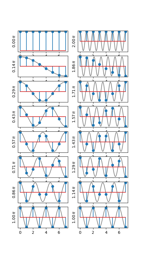
Fig. 3.7 Frequency symmetry in the discrete time complex exponentials. In the left column the frequency \(\W\) runs from \(0\) to \(\pi\) going top to bottom. In the right column the frequency is \(2\pi-\W\) where \(\W\) is the frequency in the same row in the left column (so for both plots on the bottom row the frequency is \(\W=\pi\). In blue the DT signal \(x[n]=\cos(\W n)\) is shown, in gray the CT signal \(x(t)=\cos(\W t)\) is shown (assuming the sampling time is 1 s).
As an example of the DT Fourier transform consider a discrete block function of 5 samples:
\[\begin{split}b_2[n] = \begin{cases} 1 &: |n|\leq 2\\ 0 &: |n|>2 \end{cases}\end{split}\]
Its Fourier transform can be calculated as:
\[\begin{split}B(\W) &= e^{-2j\W} + e^{-j\W} + 1 + e^{j\W} + e^{2j\W}\\ &= 1 + 2 \cos(\W) + 2 \cos(\W n)\end{split}\]
Show code for figure
 1import numpy as np
 2import matplotlib.pyplot as plt
 3from matplotlib.ticker import FuncFormatter, MultipleLocator
 4
 5plt.close('all')
 6
 7
 8def b2(n):
 9    return 1.0 * np.logical_and(n>=-2, n<=2)
10
11
12def B2(W):
13    return 1 + 2 * np.cos(W) + 2 * np.cos(2*W)
14
15
16fig, axs = plt.subplots(2)
17n = np.arange(-7,8)
18W = np.linspace(0, 2*np.pi, 1000)
19
20axs[0].stem(n, b2(n))
21axs[0].set_xlabel("n")
22axs[0].set_ylabel('$b_2(n)$')
23
24axs[1].plot(W, B2(W))
25axs[1].axhline(0)
26axs[1].set_xlabel("$\\Omega$")
27axs[1].set_ylabel('$B_2(\Omega)$')
28axs[1].xaxis.set_major_formatter(FuncFormatter(lambda val,pos: '{:.1f}$\pi$'.format(float(val)/np.pi) if val !=0 else '0'))
29axs[1].xaxis.set_major_locator(MultipleLocator(base=np.pi/2))
30
31
32plt.savefig('source/figures/blockDTNP.png')
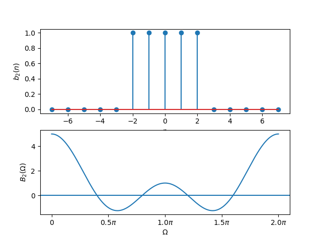
Fig. 3.8 A DT block function and its DT Fourier Transform.
Observe that the DT Fourier transform has a period of \(2\pi\). Furthermore observe that the interval \(\W\in[0,\pi]\) characterizes the entire function (for real signals…). These properties are proven in the next subsection.
3.3.2. Properties of the DTFT
Time Domain |
Frequency Domain |
|---|---|
Synthesis (Inverse Fourier Transform)
\[x[n] = \frac{1}{2\pi} \int_{\langle 2\pi \rangle} X(\Omega) e^{j\Omega n} d\Omega\]
|
Analysis (Fourier Transform)
\[X(\Omega) = \sum_{n=-\infty}^{\infty} x[n] e^{-j \Omega n}\]
|
Real Signals
\[x[n] \in\setR\]
|
Symmetry in Fourier transform
\[X(-\Omega) = X^\star(\Omega)\]
|
Even Signals
\[x[-n] = x[n]\]
|
Real Fourier transform
\[X(\Omega) \text{ is real}\]
|
Odd Signals
\[x[-n] = -x[n]\]
|
Imaginary Fourier transform
\[X(\Omega) \text{ is imaginary}\]
|
Time Shift
\[x[n-n_0]\]
|
Phase factor
\[e^{-j \W n_0} X(\W)\]
|
Difference
\[x[n] - x[n-1]\]
|
\[(1-e^{-j \Omega})X(\Omega)\]
|
Convolution
\[x[n] \ast y[n]\]
|
Multiplication
\[X(\Omega) Y(\Omega)\]
|
Multiplication
\[x[n] y[n]\]
|
Convolution
\[\frac{1}{2\pi} X(\w)\ast_{\langle 2\pi\rangle} Y(\Omega)\]
|
Real Signals
Let \(x(t)\) be a real signal then \(X(-\Omega)=X^\star(\Omega)\). The proof immediately follows from the definition.
Symmetry
Consider the frequency in the range from \(\pi\) to \(2\pi\). The value of \(X(\Omega)\) for these frequencies for real signals is not really neaded due to summetry (periodicity)
\[\begin{split}X(2\pi-\Omega) &= \sum_{n=-\infty}^{\infty} x[n]e^{-j (2\pi - \Omega) n}\\ &= \sum_{n=-\infty}^{\infty} x[n]e^{-j 2\pi n}e^{ j\Omega n}\\\end{split}\]
Note that \(e^{-j2\pi n}=1\) for all \(n\). So for a real valued signal \(x[n]\) we have:
\[\begin{split}X(2\pi-\Omega) &= \sum_{n=-\infty}^{\infty} x[n] e^{j\Omega n}\\ &= X(-\Omega)\\ &= X^\star(\Omega)\end{split}\]
In summary we only need to consider the \(X(\Omega)\) values for \(0\leq\Omega<\pi\).
Shift in Time Domain
A shift in the time domain corresponds with a phase shift in the frequency domain:
\[x[n-n_0] \FTright e^{-j\Omega n_0} X(\Omega)\]
The proof is simple. Take \(x[n-n_0]\) into the definition of DTFT:
\[\FT(x[n-n_0]) = \sum_{n=-\infty}^{\infty} x[n-n_0] e^{-j\Omega n}\]
substituting \(n'=n-n_9\) we get:
\[\begin{split}\FT(x[n-n_0]) &= \sum_{n'=-\infty}^{\infty} x[n'] e^{-j\Omega (n'+n_0)}\\ &= \sum_{n'=-\infty}^{\infty} x[n'] e^{-j\Omega n'} e^{-j \Omega n_0}\\ &= e^{-j \Omega n_0} \sum_{n'=-\infty}^{\infty} x[n'] e^{-j\Omega n'}\\ &= e^{-j \Omega n_0} X(\Omega)\end{split}\]
Shift in Frequency Domain
The dual property of the shift in time domain is the shift in the frequency domain:
\[e^{j\Omega_0 n} x[n] \FTright X(\Omega-\Omega_0)\]
The proof is simple, just calculate the Fourier transform of \(e^{j\W_0 n}x[n]\) following the definiion.
Convolution in Time Domain
Convolution in the time domain corresponds with multiplication in the frequency domain.
\[x[n]*y[n] \FTright X(\Omega)Y(\Omega)\]
The proof is straightforward. We have:
\[\begin{split}\FT\{x[n]\ast y[n]\} &= \FT\left\{ \sum_{k=-\infty}^{\infty} x[n-k] y[k] \right\}\\ &= \sum_{k=-\infty}^{\infty} \FT\{x[n-k]\} y[k]\\ &= \sum_{k=-\infty}^{\infty} e^{-j\W k} X(\W) y[k]\\ &= X(\W) \sum_{k=-\infty}^{\infty} y[k] e^{-j\W k}\\ &= X(\W) Y(\W)\end{split}\]
Multiplication in Time Domain
Difference in Time Domain
In the discrete time domain we cannot calculate the derivative of a signal \(x[n]\) (it can be done only in approximation). De difference operator \(y[n]=x[n]-x[n-1]\) is the best we can locally do to estimate the derivative. For the Fourier Transform we have:
Straigtforward use of the linearity of the Fourier transform and one of its properties we get:
3.3.3. Fourier Transform Pairs
As with all Fourier transforms we list some of the important Fourier transform pairs.
Time Domain |
Frequency Domain |
|---|---|
Synthesis (Inverse Fourier Transform)
\[x[n] = \frac{1}{2\pi} \int_{\langle 2\pi \rangle} X(\Omega) e^{j\Omega n} d\Omega\]
|
Analysis (Fourier Transform)
\[X(\Omega) = \sum_{n=-\infty}^{\infty} x[n] e^{-j \Omega n}\]
|
Pulse
\[x[n]=\delta[n]\]
|
Constant
\[X(\W) = 1\]
|
Step
\[\begin{split}u[n] = \begin{cases}1 &: n\geq 0\\ 0 &: n<0\end{cases}\end{split}\]
|
\[\frac{1}{1-e^{-j\W}} + \pi\sum_{k=-\infty}^{+\infty} \delta(\W-2k\pi)\]
|
Block
\[\begin{split}b_N[n] = \begin{cases}\frac{1}{N} &: 0\leq n < N\\ 0 &:\text{elsewhere}\end{cases}\end{split}\]
|
\[B_N(\W) = \frac{1}{N}\frac{1-e^{-j\W N}}{1-e^{-j\W}}\]
|
Complex Exponential
\[e^{j\W_0 n}\]
|
\[2\pi \sum_{k=-\infty}^{\infty} \delta(\W - \W_0 + k 2\pi)\]
|
Step Function
The proof for the Fourier transform of the step function is not trivial. There are many video’s to be found explaining the proof (where the step function is written as the sum of a constant and a sign function). The constant then gives rise to the pulse function in the Fourier transform.
Block Function
The block function \(b_N[n]\) as defined in the table above, can be written as the difference of two shifted step functions:
For the discrete Fourier transform of \(b_N\) we can use the transform of the step function and the shifted step function. Another way of calculating the discrete Fourier transform if by writing \(b_N\) as the finite sum of shifted pulses and using the sum formula for a geometric sequence (see the chapter on Geometric Sequences).
Complex Exponential
The proof for the complex exponential is relatively simple when we substite \(X(\W)\) into the synthesis equation and derive the complex exponential function.
Substituting
leads to
Due to the integration over only a period of \(2\pi\) we can reduce the summation to just the term for \(k=0\) and get:
3.3.4. Introducing Time
Thusfar we have not used time, a discrete signal \(x[n]\) doesn’t refer to time. But now let us introduce time in the following way:
i.e. each value \(x[n]\) is the value of the CT signal \(x(t)\) at time \(t=nT_s\) where \(T_s\) is the sample period.
We have allready seen that the highest frequency corresponding with \(\Omega = \pi\) corresponds with a block wave (square wave) with period \(2T_s\) and thus with frequency \(1/(2T_s)\). So we can link the radial frequency \(\Omega\) with the time domain frequency \(f\):
The radial frequency we know from CT systems is \(\w = 2\pi f\) and thus
Note that you should only use these for \(0\leq\Omega\leq\pi\).
3.3.5. Exercises
- Fourier Transform
Given the signal:
\[\begin{split}x[n] = \begin{cases} 1 &: n=-1\\ -1 &: n=0\\ 1 &: n=1\\ 0 &: \text{elsewhere} \end{cases}\end{split}\]Calculate the Fourier transform \(X(\Omega)\)
Plot the frequency spectrum \(X(\Omega)\)
- Convolution
Given two Fourier transforms:
\[\begin{split}X_1(\Omega) &= 1 + 2 e^{-j\Omega} + 4 e^{-j 2\Omega}\\ X_2(\Omega) &= 2 + e^{-j\Omega}\end{split}\]Give \(x_1[n]\) and \(x_2[n]\)
Calculate the convolution of \(y[n] = x_1[n] \ast x_2[n]\)
Calculate \(Y(\Omega)\) from the result above (i.e. using \(y[n]\)).
Calculate \(Y(\Omega)\) using the convolution property.
- Zero Response
Consider the discrete convolution kernel function
\[\begin{split}h[n] = \frac{1}{7} \begin{cases} 1 &: |n|\leq 3\\ 0 &: \text{elsewhere} \end{cases}\end{split}\]and the signal \(x[n]\):
\[x[n] = \sin(\W_0 n)\]Calculate the DTFT \(H(\W)\) of \(h[n]\).
Calculate the DTFT \(X(\W)\) of \(x[n]\).
For which values of \(\W_0\) is the response zero, i.e. \(\forall n:\; x[n]\ast h[n] = 0\).