5.5.2. Block Diagrams

In signal processing and control a lot of the systems are visualized as block diagrams. A block represents a (linear) system and arrows indicate the signals flowing from block to block starting at the input and ending at the output of the system.

In this chapter we consider the block diagrams of linear time invariant systems characterized in the s-domain. Similar block diagrams can be used for discrete systems (see the chapter on filters).

5.5.2.1. Cascade of Systems

Let a signal \(x(t)\) be fed into a system with transfer function \(H_1(s)\). The output \(y(t)\) of this system is then fed into a second system with transfer function \(H_2(s)\). Let \(z(t)\) be the output of the second system.

The signal flow characterized in the s-domain is:

\[X(s) \longrightarrow Y(s) = H_1(s) X(s) \longrightarrow Z(s) = H_2(s) Y(s) = H_1(s)H_2(s) X(s)\]

Thus the transfer function for the entire system is:

\[H(s) = \frac{Z(s)}{X(s)} = H_1(s) H_2(s)\]

Cascading LTI systems thus amounts to a multiplication of the separate transfer functions.

5.5.2.2. Addition of System outputs

Consider the system that contains two subsystems \(H_1(s)\) and \(H_2(s)\) each processing the same input \(X(s)\). The outputs of both systems are added to give the result \(Y(s)\). Evidently we have:

\[H(s) = \frac{Y(s)}{X(s)} = H_1(s) + H_2(s)\]

5.5.2.3. Feedback Systems

What we will often use in control systems is the feedback loop. Here we will use the output value itself in the calculation of the output. Consider the following system:

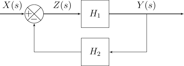
Fig. 5.50 Negative Feedback Loop

Observe that

\[Y(s) = Z(s)H_1(s)\]

and also

\[Z(s) = X(s) - H_2(s)Y(s)\]

Using the first expression for \(Y(s)\) the above equation can be rewritten as:

\[X(s) = Z(s) + Z(s) H_1(s) H_2(s)\]

Now combining the first expression for \(Y(s)\) with the last one for \(X(s)\) we get:

\[\frac{Y(s)}{X(s)} = \frac{Z(s)H_1(s)}{Z(s)+Z(s)H_1(s)H_2(s)} = \frac{H_1(s)}{1+H_1(s)H_2(s)}\]

Although not difficult to derive, this equation is worth memorizing as it will be used over and over again in control systems.

A somewhat simpler way to derive the same expression is noting that:

\[Y(s) = H_1(s) \bigl( X(s) - H_2(s) Y(s) \bigr)\]

and thus:

\[\bigl( 1 + H_1(s) H_2(s)\bigr) Y(s) = H_1(s) X(s)\]

leading to:

\[H(s) = \frac{Y(s)}{X(s)} = \frac{H_1(s)}{1+H_1(s)H_2(s)}\]

For now a feedback system is just a peculiarity but in subsequent sections we will show that feedback systems are very important in engineering science.