3.1. Continuous Time Fourier Series

The CT Fourier Series considers periodic signals. A signal \(x(t)\) is periodic with period \(T\) in case:

\[\forall t:\quad x(t+T) = x(t)\]

Note that in case \(x\) is periodic with period \(T\) it is also periodic with period \(2T\) (or \(nT\)). This leads us to the definition of the fundamental period (\(T_0\)) being the smallest value such that \(x(t+T_0)=x(t).\) The fundamental frequency then is \(f_0=1/T_0\).

3.1.1. The Complex Exponential Functions

We have already introduced the complex exponential functions \(x(t) = e^{j \w t}\). This function is periodic with period \(T = \frac{2\pi}{\w}\). If we fix \(\omega\), say at value \(\omega_0\) then the fundamental period is \(T_0=2\pi/\omega_0\). The functions \(x(t)=\exp(j k\omega_0 t)\) for integer \(k>0\) then are all \(T_0\) periodic, in fact the period for \(\exp(j k\omega_0)\) is:

\[T_k = \frac{2\pi}{k\omega_0} = \frac{T_0}{k}\]

Consider only the imaginary part of the complex exponential for illustration purposes:

\[\sin(k \omega_0 t) = \sin\left(\frac{2 k \pi}{T_0} t\right)\]

for different values of \(k>0\). We see that these sine functions fit exactly \(k\) times in the interval of length \(T_0\).

Show code for figure

import numpy as np
import matplotlib.pyplot as plt

plt.clf()
T0 = 10
t = np.linspace(0,T0,1000)

K = 5
fig, axs = plt.subplots(nrows=K, sharex=True)
for k in range(1,K+1):
    axs[k-1].plot(t, np.sin(2*k*np.pi*t / T0))

plt.savefig('source/figures/sines.png')

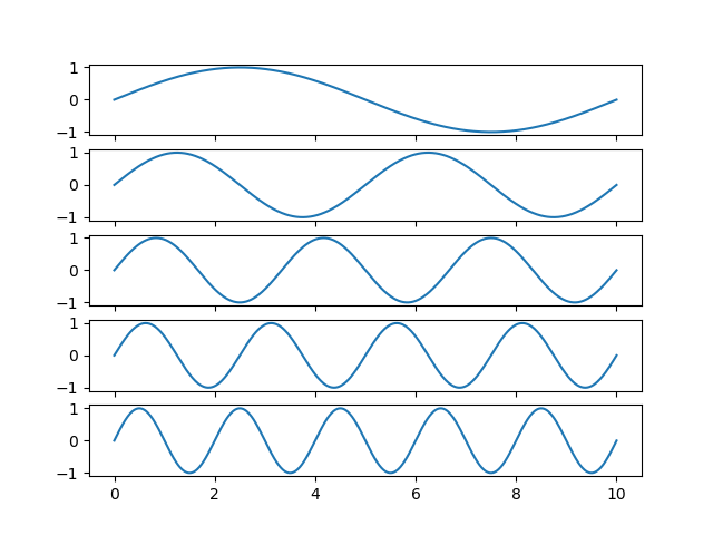
Fig. 3.1 Harmonics. The sine function at fundamental frequence \(\w_0\) and the harmonics at frequencies \(2\w_0\), \(3\w_0\), \(4\w_0\) and \(5\w_0\).

The fundamental (lowest) frequency of the sinusoidal signal is \(\omega_0\) and the frequencies \(k\omega_0\) for \(k>1\) are called the harmonics, \(k=1\): first harmonic, etc. Why this set of periodic signals is so important has been discovered by Fourier and is the subject of the next subsection.

3.1.2. The Fourier Series

Fourier (a French mathematician) showed that nearly every periodic function (with period \(T_0\)) can be written as a linear combination (superposition) of the complex exponential functions \(\exp(j k \omega_0 t)\) for \(k=0,1,2,\cdots\) where \(\omega_0 = 2\pi / T_0\):

\[x(t) = \sum_{k=-\infty}^{\infty} a_k e^{ j k \omega_0 t}\]

Note that the coefficients determining the weight of every frequency \(k\omega_0\) in general are complex valued.

As an example consider the periodic function \(x(t)\) with period \(T_0\):

\[\begin{split}x(t) = \begin{cases} 1 &: 0\leq t <T_0/2\\ 0 &: T_o/2 \leq t < T_0 \end{cases}\end{split}\]

Note that we only defined the periodic function on one of its periods. The function has the entire real axis as its domain.

This function can be written as the sum of complex exponentials with:

\[\begin{split}a_0 &= 1/2\\ a_k &= \frac{1}{j k 2\pi} (1-e^{-j k \pi}) \quad \text{for } k\geq 1\end{split}\]

Show code for figure

plt.clf()

T0 = 4

def f(t):
    return ((t % T0)<=0.5*T0).astype('float')

t = np.linspace(-0.2,1.7*T0,1000)
x = f(t)

def phi(t, k):
    if k==0:
          return 1/2 * np.ones_like(t)
    return -1j / (2 * k * np.pi) * (1 - np.exp(-1j*k*np.pi)) * np.exp( 1j * k * 2 * np.pi / T0 * t)

K = 11
xa = phi(t,0)

for k in range(1,K,2):
    xak = phi(t,k)+phi(t,-k)
    xa = xa + xak
    plt.subplot(K,2,2*k+1)
    plt.plot(t,x,lw=1)
    plt.plot(t,xak,lw=2)
    plt.axis('off')
    plt.axis([-0.2, 1.7*T0, -0.8, 1.2])
    plt.subplot(K,2,2*k+2)
    plt.plot(t,x,lw=1)
    plt.plot(t,xa,lw=2)
    plt.axis('off')
    plt.axis([-0.2, 1.7*T0, -0.8, 1.2])

plt.savefig('source/figures/fourierblock.png')

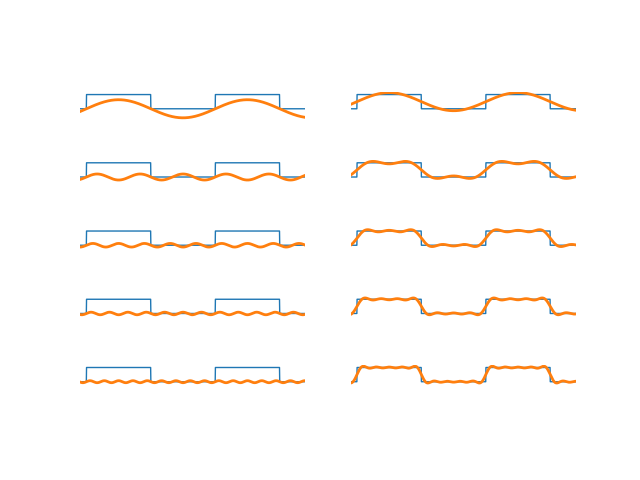
Fig. 3.2 Fourier series decomposition of block wave.

In the figure above the left column shows the functons \(a_k \exp(-j k \omega_0 t)\) starting from \(k=1\) whereas in the second column the addition of these functions from \(k=0\) upto \(k\) are shown. Note that only the odd values for \(k\) are shown as \(a_k=0\) for even \(k\). Observe that for even \(k\) we have \(a_k=0\). This will prove to be the case for any odd function \(x\).

The Fourier coefficients are given by:

\[a_k = \frac{1}{T_0} \int_{\langle T_0 \rangle} x(t) e^{-j k \omega_0 t} dt\]

Summarizing the Continuous Time Fourier Series:

Synthesis	Analysis
\[x(t) = \sum_{k=-\infty}^{\infty} a_k e^{ j k \omega_0 t}\]	\[a_k = \frac{1}{T_0} \int_{\langle T_0 \rangle} x(t) e^{-j k \omega_0 t} dt\]

We won’t give the proof of the surprising findings of Fourier leading to the synthesis equation. The proof of the analysis equation—given the synthesis equation—is a lot easier.

We start with the synthesis equation and multiply both sides with \(\exp(-j l \omega_0 t)\) (we introduce variable \(l\) not to get confused with variable \(k\) just in the summation):

\[\begin{split}x(t) e^{-j l \omega_0 t} &= \left(\sum_{k=-\infty}^{\infty} a_k e^{ j k \omega_0 t}\right) e^{-j l \omega_0 t}\\ &= \sum_{k=-\infty}^{\infty} a_k e^{ j (k-l) \omega_0 t}\end{split}\]

Now integrate both sides over a period \(T_0\):

\[\begin{split}\int_{\langle T_0 \rangle} x(t) e^{-j l \omega_0 t} dt &= \int_{\langle T_0 \rangle}\left(\sum_{k=-\infty}^{\infty} a_k e^{ j (k-l) \omega_0 t}\right)dt\\ &= \sum_{k=-\infty}^{\infty} a_k \int_{\langle T_0 \rangle} e^{ j (k-l) \omega_0 t} dt\end{split}\]

Note that the integral on the right hand side equals \(T_0\) in case \(k=l\) and the integral is equal to zero in case \(k\not=l\) (remember that integrating a sine or cosine over a multiple of its periods is always zero). So:

\[\begin{split}\int_{\langle T_0 \rangle} x(t) e^{-j l \omega_0 t} dt &= a_l \int_{\langle T_0 \rangle} dt\\ &= a_l T_0\end{split}\]

or:

\[a_l = \frac{1}{T_0} \int_{\langle T_0 \rangle} x(t) e^{-j l \omega_0 t} dt\]

So starting with the synthesis equation we arrived at the analysis equation.

Observe that the real valued function \(x\) defined on one period is equivalent with all coefficients \(a_k\) for \(k\geq0\). For a complex valued function we need all \(a_k\) for all values of \(k\). The coefficient \(a_k\) for a real valued function \(x\) is associated with a sinusoidal function of frequency \(k\w_0\) where \(\w_0=2\pi/T_0\). Plotting the values \(a_k\) as a function of the (radial) frequency \(\w\) is known as the (discrete) frequency spectrum.

For the block function plotted above, the frequency spectrum looks like:

Show code for figure

plt.clf()

a = np.zeros(11, dtype=complex)
a[0] = 1/2;
for k in range(1,11):
    a[k] = -1j / (2 * k * np.pi) * (1 - np.exp(-1j*k*np.pi))

#print(a, file=sys.stderr)

plt.stem(np.arange(11), np.abs(a), use_line_collection=True)
plt.xlabel(r'$k$')
plt.ylabel(r'$|a_k|$')

plt.savefig('source/figures/ctfsspectrum.png')

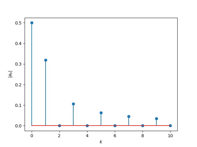
Fig. 3.3 Frequency spectrum of block wave function.

Note that the amplitude of the higher frequency sinusoids are are getting less and less. Evidently the plot above should be accompanied with a plot of \(\angle a_k\). We leave that as an exercise to the reader.

3.1.3. Properties of the CT Fourier Series

In this subsection we give some properties of the CT Fourier series. In later subsections we will prove a lot of these properties.

Time Domain	Frequency Domain
Synthesis \[x(t) = \sum_{k=-\infty}^{\infty} a_k e^{ j k \omega_0 t}\]	Analysis \[a_k = \frac{1}{T_0} \int_{\langle T_0 \rangle} x(t) e^{-j k \omega_0 t} dt\]
Real Signal \[x(t) \in \setR\]	Complex Conjugates \[a_{-k} = a_k^\star\]
Even Signal \[x(-t) = x(t)\]	Real Coefficients \[a_k \text{is real}\]
Odd Signal \[x(-t) = -x(t)\]	Imaginary Coefficients \[a_k \text{is imaginary}\]
Derivative \[\begin{split}x'(t) &= \frac{d}{dt} x(t)\\ x^{(n)}(t) &= \frac{d^n}{dt^n} x(t)\end{split}\]	High Frequency Gain \[\begin{split}j k \omega_0 a_k\\ \left(j k \omega_0\right)^n a_k\end{split}\]
Convolution \[\begin{split}x(t)\\ y(t)\\ x(t) \ast y(t)\end{split}\]	Multiplication \[\begin{split}a_k\\ b_k\\ T_0 \; a_k \; b_k\end{split}\]
Multiplication \[x(t) y(t)\]	Convolution \[T_0 \sum_{l=-\infty}^{\infty} a_l\; b_{k-l}\]

3.1.3.1. Real Valued Signal

In signal processing we are most often working with real valued signals. For such a real valued signal we have:

\[a_k = a^\star_{-k}\]

This is not too difficult to prove. First the synthesis equation can be rewritten such that we ‘unroll the summation loop’:

\[x(t) = a_0 + \sum_{k=1}^{\infty} \left( a_{-k} e^{ - j k \omega_0 t} + a_k e^{ j k \omega_0 t} \right)\]

Using Euler’s formula and writing \(a_k=A_k+jB_k\) where \(A_k\) and \(B_k\) are real\int_{-\infty}^{\infty} x(t) e^{-j\w t} dt numbers, we get:

\[x(t) = a_0 + \sum_{k=1}^{\infty} \left( (A_{-k}+jB_{-k}) (\cos(k\omega_0 t) - j\sin(k\omega_0 t)) + (A_k+jB_k) (\cos(k\omega_0 t) + j\sin(k\omega_0 t)) \right)\]

Collecting real and imaginary parts leads to:

\[\begin{split}x(t) = a_0 + \sum_{k=1}^{\infty} \left( (A_{-k} + A_k)\cos(k\omega_0 t) + (B_{-k}-B_k)\sin(k\omega_0 t) \right) + \\ j \sum_{k=1}^{\infty} \left( (B_{-k}+B_k)\cos(k\omega_0 t) + (-A_{-k} + A_k)\sin(k\omega_0 t) \right)\end{split}\]

The imaginary part of the above equation can only be zero (what we need for a real signal) in case:

\[\begin{split}A_{-k} = A_k\\ B_{-k} = - B_k\end{split}\]

Both of these make \(a_{-k} = a^\star_k\).

So we can write:

\[x(t) = a_0 + 2 \sum_{k=1}^{\infty} \left( A_k \cos(k\omega_0 t) - B_k \sin(k\omega_0 t) \right)\]

Remember from high school trigonometry that a summation of a sine and cosine of the same frequency results in a shifted sine:

\[x(t) = a_0 + 2 \sum_{k=1}^{\infty} |a_k| \sin(k\omega_0 t - \angle a_k)\]

This last synthesis equation shows that a periodic real valued function can be written as the sum of sine functions of frequency \(k\omega_0\) for \(k>0\).

3.1.3.2. Even Signal

For an even signal, i.e. \(x(-t)=x(t)\) we have:

\[a_k \text{is real}\]

The proof is not to difficult. We start with the definition

\[a_k = \frac{1}{T_0} \int_{\langle T_0 \rangle} x(t) e^{-j k \omega_0 t} dt\]

If we make a choice for the interval \(t\in[-T_0/2, T_0/2]\) we get

\[\begin{split}a_k &= \frac{1}{T_0} \int_{t=-T_0/2}^{T_0/2} x(t) e^{-j k \omega_0 t} dt\\ &= \frac{1}{T_0} \int_{t=0}^{T_0/2} (x(t)+x(-t)) e^{-j k \omega_0 t} dt\\ &=\end{split}\]

3.1.3.3. Odd Signal

For an odd signal, i.e. \(x(-t)=-x(t)\) we have:

\[a_k \text{is imaginary}\]

3.1.3.4. Differentiation

Consider a periodic CT signal \(x(t)\) and its corresponding Fourier series coefficients \(a_k\). We have that derivate signal \(x'(t)\) has Fourier series coefficients \(jk\omega_0 a_k\).

This is really easy to prove:

\[x(t) = \sum_k a_k e^{j k \omega_0 t}\]

and thus differentiating both sides leads to

\[\begin{split}x'(t) &= \sum_k a_k \frac{d}{dt} e^{j k \omega_0 t} \\ &= \sum_k a_k\, j k \omega_0 \, e^{j k \omega_0 t}\end{split}\]

Let \(x^{(n)}\) denote the \(n\)-th order derivative of \(x\) then the Fourier series coefficients of \(x^{(n)}\) are equal to \((jk \omega_0)^n \, a_k\).

3.1.3.5. Convolution

Let \(x\) be a CT periodic signal with period \(T_0\). Then convince yourself that the convolution \(x\ast y\) on the infinite domain for any function \(y\) is periodic too. Relating this convolution to the Fourier series is hard (i think…), most often we restrict the analysis of convolutions to functions \(y\) that are \(T_0\)-periodic as well.

In this case the convolution is defined as:

\[(x \ast_{T_0} y)(t) = \int_{\langle T_0 \rangle} x(u)y(t-u) du\]

i.e. it is restricted to one period of length \(T_0\).

Let \(a_k\) be the Fourier coefficients of \(x\) and \(b_k\) be the coefficients for \(y\) then the coefficients for \(x\ast_{T_0} y\) are \(T_0 a_k b_k\).

The proof is not too complicated. It is a nice way to exercise your integration skills (see https://math.stackexchange.com/questions/97328/f-g-continuous-and-periodic-functions-with-1-prove-periodic-widehat-fg?rq=1)

3.1.3.6. Fourier Series Examples

3.1.3.6.1. Block Wave Function

We start with the simple block wave function that we have allready seen in the beginning of this section:

\[\begin{split}x(t) = \begin{cases} 1 &: 0\leq t <T_0/2\\ 0 &: T_o/2 \leq t < T_0 \end{cases}\end{split}\]

The Fourier coefficients are calculated as:

\[\begin{split}a_k &= \frac{1}{T_0} \int_{\langle T_0 \rangle} x(t) e^{-j k \omega_0 t} dt \\ &= \frac{1}{T_0} \int_{0}^{T_0/2} e^{-j k \omega_0 t} dt\end{split}\]

For \(k=0\) the integrand is 1 and thus:

\[a_0 = \frac{1}{2}\]

For \(k\not=0\) we have

\[\begin{split}a_k &= \frac{1}{T_0} \left[ \frac{1}{- j k \omega_0} e^{-j k \omega_0 t} \right]_0^{T_0/2} \\ &= \frac{1}{T_0} \frac{1}{j k \omega_0} \left( 1 - e^{-j k\w_0 T_0/2} \right)\end{split}\]

Remember that \(\w_0 = 2\pi/T_0\) and thus for \(k\not=0\):

\[a_k = \frac{1}{j k 2\pi} \left( 1 - e^{-j k\pi} \right)\]

For even \(k\) we have \(e^{-jk\pi}=1\) and thus \(a_k=0\). For odd \(k\) we have \(e^{-jk\pi}=-1\) leading to

\[\begin{split}a_k = \begin{cases} \half &: k=0\\ 0 &: k \text{ is even}\\ \frac{1}{j k \pi} &: k \text{ is odd} \end{cases}\end{split}\]

3.1.3.6.2. From Time Domain to Frequency Domain

Consider the time signal \(x(t) = 1 + \sin(2t) + \cos(3t)\). The Fourier coefficients can again be calculated with the analysis equation. However in this case it is much easier to rewrite the given equation for \(x\) into a form that is close to the synthesis equation.

\[\begin{split}x(t) &= 1 - \half j (e^{2jt}-e^{-2jt}) + \half (e^{3jt}+e^{-3jt}) \\ &= \half e^{-3jt} +\half j e^{-2jt} + 1 - \half j e^{2jt} + \half e^{3jt}\end{split}\]

From which we can immediately conclude (without doing any integrations):

\[\begin{split}a_{-3} &= \half \\ a_{-2} &= \half j\\ a_0 &= 1\\ a_2 &= -\half j\\ a_3 &= \half\end{split}\]

All other \(a_k\)’s are zero.

Note: in case you really feel like using the analysis equation and do the integrations by hand you should first determine the period \(T_0\) of this signal. For \(\sin(2t)\) the period is \(\pi\), for \(\sin(3t)\) the period is \(\tfrac{2}{3}\pi\). Be sure to understand that for \(x(t)\) the period is \(T_0=2\pi\).

3.1.3.6.3. Triangular Signal

We define the triangular signal \(x(t)\) as shown in the figure below.

Show code for figure

plt.clf()

t = np.linspace(-0.2, 1.7, 1000)
tm1 = t % 1
x = np.piecewise(tm1, [tm1<=0.5, tm1>0.5], [lambda t: -1/8+1/2*t, lambda t: 3/8 - 1/2*t])
plt.plot(t,x)
plt.savefig('source/figures/trianglesignal.png')

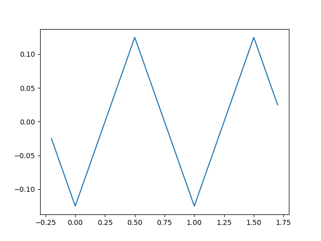
Fig. 3.4 Triangular signal.

Observe that the derivative \(x'(t)\) of \(x(t)\) is the block function that we have discussed in the first exercise (except that for \(x'(t)\) we have \(a_0=0\) (you should be able to conclude that without calculation). For all other Fourier coefficients we have (according to the derivative rule):

\[a'_k = jk\w_0 a_k\]

where the \(a'_k\)’s are the Fourier coefficients of the derivative signal. The derivative is the familiar block function with Fourier coefficients:

\[\begin{split}a'_k = \begin{cases} 0 &: k \text{ is even, including }0\\ \frac{1}{j k \pi} &: k \text{ is odd} \end{cases}\end{split}\]

So for the triangular signal we have:

\[a_k = \frac{a'_k}{j k \w_0} = \frac{T_0}{j k 2\pi} a'_k = \frac{1}{j k 2\pi} a'_k\]

leading to:

\[\begin{split}a_k = \begin{cases} 0 &: k \text{ is even, including }0\\ \frac{-1}{2 k^2 \pi^2} &: k \text{ is odd} \end{cases}\end{split}\]

Using the synthesis equation we can applximately reconstruct the triangle signal using a few of the harmonics.

Show code for figure

plt.clf()

def ak(k):
    if k%2 == 0:
        return 0
    return -1/(2 * k**2 * np.pi**2)

def phi(t,k):
    return ak(k) * np.exp(1j * k * 2 * np.pi * t)

def Phi(t,k):
    r = np.zeros_like(t, dtype=complex)
    for i in range(-k, k+1):
        r += phi(t,i)
    return r.real

plt.subplot(3,1,1)
plt.plot(t, x)
plt.plot(t, Phi(t,1))
plt.subplot(3,1,2)
plt.plot(t, x)
plt.plot(t, Phi(t,3))
plt.subplot(3,1,3)
plt.plot(t, x)
plt.plot(t, Phi(t,5))
plt.savefig('source/figures/trianglesignalharmonics.png')

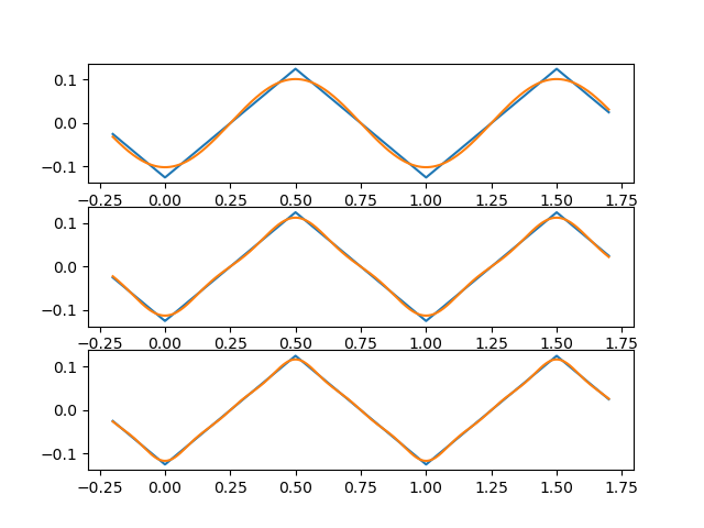
Fig. 3.5 Triangle wave signal and its harmonics. In blue the triangular signal in red the reconstruction using a few harmonics. Top row: \(|k|\leq1\), middle row: \(|k|\leq3\) and bottom: \(|k|\leq5\).

3.1.4. Exercises

1. Parabolic Function

   Consider the function \(x(t)\) defined on the interval from 0 to 1 (and periodically continuated)

   \[x(t) = t^2\]

   1. Calculate the Fourier coefficients \(a_k\). The use of Mathematica or Wolfram alpha or Maple or … is allowed here.

   2. Plot both \(|a_k|\) and \(\angle(a_k)\) as a function of \(k\).

2. Frequency and Period

   For each of the following functions calculate radial frequenct \(\w\) and the period \(T\)

   1. \(\sin(t)\)

   2. \(\cos(3t)\)

   3. \(\sin(\half t)\)

   4. \(\sin(\pi/3 t)\)

   5. \(\sin(0.4 t)\)

3. Fundamental Frequency and Period

   Below several functions of the form \(x(t)=x_1(t)+x_2(t)\) are given. For each of them calculate the frequency \(\w_1\) and period \(T_1\) of \(x_1\), the same for \(x_2(t)\) and the same 1.or \(x(t)=x_1(t)+x_2(t)\)

   1. \(x_1(t) = \sin(t),\quad x_2(t)=2\cos(t)\)

   2. \(x_1(t) = \sin(t), \quad x_2(t) = \cos(t + \pi)\)

   3. \(x_1(t) = \sin(2t), \quad x_2(t) = 0.5 \cos(3t)\)

   4. \(x_1(t) = \sin(0.5t), \quad x_2(t) = 2 \sin(3t)\)

   5. \(x_1(t) = \sin(6t), \quad x_2(t) = \cos(10t)\)

   6. \(x_1(t) = \sin(8t), \quad x_2(t) = 2\sin(12t)\)

   7. \(x_1(t) = \sin(66t), \quad x_2(t) = \cos(77t)\)

   8. \(x_1(t) = \sin(0.3t), \quad x_2(t) = 0.5\cos(4t)\)

   9. \(x_1(t) = \sin(t), \quad x_2(t) = \sin(3\pi t)\)

4. Periodic Signal

   Given the following periodic signal \(x(t)=\sum_{k=-3}^{3} a_k e^{j k t}\) with \(a_0=1, a_{\pm 1} = 1/4, a_{\pm 2}=1/2, a_{\pm 3}=1/3\)

   1. What is the period \(T\) and fundamental frequency \(\w\).

   2. Write \(x(t)\) as a sum of sinusoids.

5. Periodic Block Signal

   Given the periodic function \(x(t)\) for one period:

   \[\begin{split}x(t) = \begin{cases} 1 &: -\frac{\pi}{2}\leq t < \frac{\pi}{2}\\ 0 &: \frac{\pi}{2} \leq t < \frac{7 \pi}{2} \end{cases}\end{split}\]

   1. What is the period and fundamental frequency?

   2. Calculate \(a_k\) for all \(k\in\setZ\).

   3. Plot the amplitude spectrum (i.e. \(|a_k|\) as function of \(k\)).

   4. Why are all \(a_k\) real?