2. Linear Time Invariant Systems

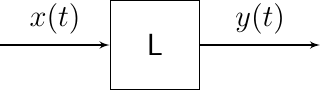
In this section we consider systems that take one input system \(x(t)\) and produce one output signal \(y(t)\). Furthermore we will consider linear time invariant systems. Given an input signal \(x\) the output is \(y=\op L x\).

Fig. 2.1 A one input, one output shift invariant linear system.

In this chapter we will learn that a LTI system (which will be defined in the first subsection of this chapter) can be (completely) characterized in several ways:

1. Impulse Response. If we provide an impulse function as input to the system, i.e. \(x(t)=\delta(t)\) for CT system, the output \(y(t)=h(t)\), where \(h(t)\) is called the impulse response function, completely characterizes the system.

   Show code for figure

   import numpy as np
   import matplotlib.pyplot as plt
   import control
   
   fig, (axin, axout) = plt.subplots(ncols=2, sharey=True, figsize=(10,3))
   fig.tight_layout()
   t = np.linspace(-2, 15, 100)
   x = np.zeros_like(t)
   axin.plot(t, x, 'b')
   axin.stem([0], [1], markerfmt='^b', linefmt='blue', use_line_collection=True)
   axin.set_title('Input = impulse')
   
   P = control.tf([1], [1,1,1])
   (tim, h) = control.impulse_response(P, np.linspace(0, 15, 100))
   axout.plot(tim, h, 'b')
   tlt0 = t[t<0]
   axout.plot(tlt0, np.zeros_like(tlt0), 'b')
   axout.set_title('Output = impulse response')
   
   plt.savefig('source/figures/lti_impulse.png')
   

   

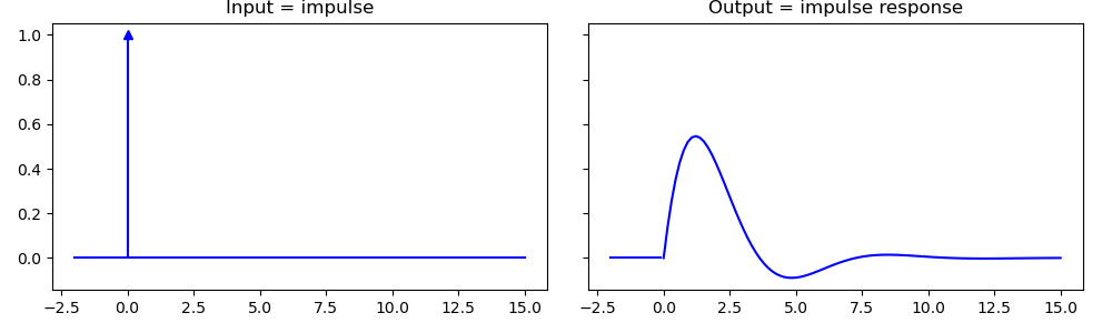
   Fig. 2.2 Impulse response.

2. Step Response. Although the impulse response completely characterizes an LTI system it is not always a practical way to identify a system. For instance consider the system of a vessel full of water that is heated with an electrical heater. Taking the temperature of the water as the output of the system and the heating power as input such a system can be approximated as an LTI system. A pulse as the input would then be a heating system that is fed with an electrical pulse of very short time duration. It is physically (nearly) impossible to have a pulse so powerful in order to raise the temperature of a large amount of water significantly. In those situations the step response is easier to work with. The step response is also a complete and unique characterization of the system. An input step in this case is a signal where until time \(t=0\) no input power is fed to the heater and from time \(t=0\) onward a constant power is fed to the system. What you will then see is that the temperature of the water will slowly increase (with an equilibrium reached when the loss of energy in the water vessel is equal to the supplied heat).

   

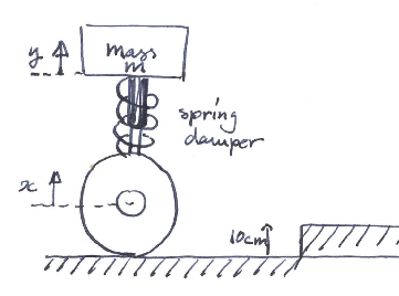
   Fig. 2.3 Mass-spring-damper system.

   Another example is a mass spring damper system (e.g. the one in a car). If you measure the height of the car above the road as the output of the system, the input signal is the road profile. Feeding this system with a pulse would be to drive over a high but very small brick in the road. Its impulse response would look a bit like the impulse response as sketched in the figure above. Driving with your car unto the pavement is like feeding this system with an input step function. Its response will look a bit like the response shown below.

   Show code for figure

   import numpy as np
   import matplotlib.pyplot as plt
   import control
   
   fig, (axin, axout) = plt.subplots(ncols=2, sharey=True, figsize=(10,3))
   fig.tight_layout()
   t = np.linspace(-2, 15, 100)
   x = np.zeros_like(t)
   x[t>=0] = 1
   axin.plot(t, x, 'b')
   axin.set_title('Input = step')
   
   P = control.tf([1], [1,1,1])
   (tim, h) = control.step_response(P, np.linspace(0, 15, 100))
   axout.plot(tim, h, 'b')
   tlt0 = t[t<0]
   axout.plot(tlt0, np.zeros_like(tlt0), 'b')
   axout.set_title('Output = step response')
   
   plt.savefig('source/figures/lti_step.png')
   

   

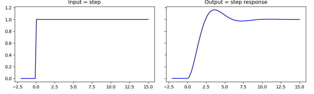
   Fig. 2.4 Step response.

3. Frequency Response. The third characteristic response of an LTI system is when the input is a periodical sine or cosine function. In this chapter we will prove that given such an input the output is again a periodical sine or cosine function, with the same frequency but with possible altered amplitude or phase (shift). The way in which the amplitude and phase of the input is altered dependent on the frequency of the input signal is called the frequency response of the system.

   Show code for figure

   import numpy as np
   import matplotlib.pyplot as plt
   import control
   
   fig, (axin, axout) = plt.subplots(ncols=2, sharey=True, figsize=(10,3))
   fig.tight_layout()
   t = np.linspace(-20, 15, 1000)
   tp = t[t>=-2]
   x = 5*np.sin(2*t)
   axin.plot(tp, x[t>=-2], 'b')
   axin.set_title('Input = sine')
   
   P = control.tf([1], [1,1,1])
   (tim, h) = control.forced_response(P, t, x)
   axout.plot(tim[tim>=-2], h[tim>=-2], 'b')
   axout.set_title('Output = damped and shifted sine')
   
   plt.savefig('source/figures/lti_freq.png')
   

   

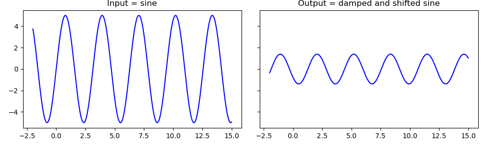
   Fig. 2.5 Frequency response. With an LTI system a sinusoidal signal is transformed into a sinusoidal signal of the same frequency. Only the amplitude and phase can be changed.

These three ways of characterizing an LTI system are equivalent. In this lecture series we will look at all three and derive the mathematical connection between the three.

• 2.1. Definition and Properties
  • 2.1.1. Linearity and Time Invariance
  • 2.1.2. Stable Systems
  • 2.1.3. Causal Systems
• 2.2. Convolutions
  • 2.2.1. Linearity + Translation Invariance = Convolution
  • 2.2.2. Properties and Recipe
• 2.3. Linear Discrete Time Systems
• 2.4. Eigenfunctions
• 2.5. Exercises