4.2.4. Difference Equations in the Z-domain
4.2.4.1. From Difference Equation to Transfer Function
A LTI system is completely characterized by its impulse response \(h[n]\) or equivalently the Z-transform of the impulse response \(H(z)\) which is called the transfer function. Remember:
Note that we thus have:
In case the impulse response is given to define the LTI system we can simply calculate the Z-transform to obtain \(H(z)\) often called the transfer function of the system.
In case the system is defined with a difference equation we could first calculate the impulse response and then calculate the Z-transform (we have done so in this section. But it is far easier to calculate the Z-transform of both sides of the difference equation.
As a first example we consider the difference equation
for which we shown that the impulse response function \(h\) is given by:
From our table of Z-transform pairs we read:
so
Instead of first finding the impulse response function of a system we could start with the difference equation and apply the Z-transform to both sides of the equation:
Rearranging terms leads to
and thus
showing that \(H(z)\) can be directly calculated from the difference equation without explicit constrution of the (infinite length) impulse response function.
As another example consider the following difference equation:
Remember that
and knowing that the Z-transform is a linear transform we can apply the Z-transform to both sides of the above equation and obtain:
This can be rewritten as:
The generic form of a difference equation is
4.2.4.2. Poles and Zeros
The generic difference equation for an LTI system is:
We have taken the number of terms (called taps in DSP lingo) both equal to \(N\). In practice some of the \(a_i\) and \(b_j\) can be zero.
Taking the Z-transform on both sides of the equation and rearranging terms leads to the transfer function \(H(z)\):
Multiplying by \(z^N/z^N\) results in
The fundamental theorem of algebra states that every \(N\)-th order complex polynomial has exactly \(N\) roots. The roots of the nominator are called the zeros of the transfer function and indinated with \(q_i\) and the roots of the denominator are called the poles of \(H\) and indinated as \(p_i\). With these zeros and poles we can rewrite the transfer function as:
The factor \(K\) expresses the fact that \(b_0\) and \(a_0\) need not be equal to one.
The zeros and poles of such a rational function in \(z\) for a system with real valued coefficients come in conjugate pairs. That is, if \(p\) is a pole then \(p^*\) is a pole as well. Also when \(z\) is a zero of \(H(z)\) then \(z^*\) is a zero as well.
A simple proof for this is as follows: Write \(H(z) = \frac{p(z)}{q(z)}\), with \(p\) and \(q\) polynomials. Then \(p\) and \(q\) must have real coefficients to get a real-valued IR filter. Write \(p(z) = a_n z^n + a_{n-1} z^{n-1} + \cdots + a_1 z + a_0\) with \(a_i \in \setR\) and let \(z_0\) be a zero of \(p\). Then \(0 = 0^* = p(z_0)^* = a_n^* (z_0^n)^* + \cdots + a_1^* z_0^* + a_0^* = a_n (z_0^*)^n + \cdots + a_1 z_0^* + a_0 = p(z_0^*)\), so \(z_0^*\) is a zero of \(p\) as well. The same holds for \(q\).
Without proof we further state the following. For a system characterized with a difference equation with real coefficients
the poles should be inside the unit circle for the system to be stable,
Any such system (arbitrary \(N\)) can be build as the cascade (sequence) of second order systems (each with \(N=2\)) and possibly a first order system \(N=1\) (in scipy.signal such a system build from at most order 2 systems is called a SOS system (Secord Order Sequence)). Note that a second order system with real coefficients has a conjugate pair of zeros and a conjugate pair of poles.
Because a LTI system is completely characterized by its transfer function \(H(z)\), the system is also completely characterized by its set of zeros and poles (together with the gain factor \(K\)). Plotting the zeros and poles in the complex plane characterizes the LTI system.
As an example consider the LTI system with transfer function \(H(z)\):
The poles and zeros are plotted in the complex plane, poles are indicated with a small cross \(\times\) and zeros are indicated with a small circle \(\circ\). In the complex plane the unit circle is also shown.
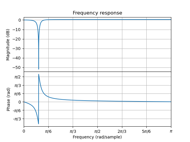
In the figure on the right the frequency response
is also shown.
Show code for figures
1import numpy as np
2import matplotlib.pyplot as plt
3from audiolazy import z
4
5H = (z**2-1.9*z+1)/(z**2-1.8*z+0.9)
6H.zplot().savefig('source/figures/hzplot.png')
7H.plot().savefig('source/figures/hfplot.png')
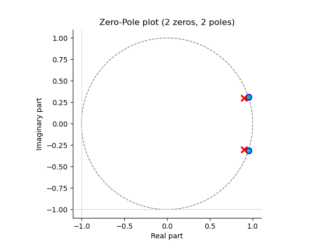
The placements of the poles and zeros determine the system (with a possible gain factor \(K\)) and thus determines the frequency response. Consider only the magnitude \(H(\W)\):
From this equation we see that if \(e^{j\W}\) is close to a zero the magnitude of the frequency response tends to be small, but if it is close to a pole its response tends to be large. In the example given zeros are exactly on the unit circle and thus the response magnitude in decibels is \(-\infty\). If \(e^{j\W}\) is further away from a zero pole pair (wich are really close to eachother) the distance to the pole and the distance to the zero are about equal and thus the influences of both cancel out (leadning to a response of 1).