3.4. Discrete Time Fourier Series

\(\newcommand{\sumN}[1]{\sum_{#1\in\langle N\rangle}}\)

As computer scientists we most often work with digital signals, i.e. DT signals. For infinite length (non periodic) signals the DT Fourier transform from the previous chapter is more of a theoretical tool to analyze DT signals and DT filters. Actually calculating the DT Fourier transform for a signal in practice is impossible as an infinite length signal cannot be stored in computer memory. let alone be processed in its entirety to calculate its Fourier transform.

In practice only a small part of a discrete signal is used to analyze its frequency components. That is where the discrete time Fourier series comes in. We start with a signal \(x[n]\) that is only defined from \(n=0\) to \(n=N-1\). This signal can be seen as one period of an infinite length signal with period \(N\) making the DTFS the discrete analog of the CT Fourier series.

The convolution kernels \(h[n]\) that are used are often defined analytically (i.e. we have a formula for it) and in many cases we are capable to calculate its discrete time Fourier transform. But for observed signals, that are defined on the infinite time axis, calculation of the Fourier transform is not feasible.

The DTFS is the transform for frequency analysis to be used in practice. It is also known as the DFT (Discrete Fourier Transform not to be confused with the Discrete Time Fourier Transform) and an efficient algorithm for the DFT is the FFT (Fast Fourier Transform). Unfortunately the choice for the normalization constants (in both the Fourier transform and its inverse) may differ. When reading articles or when using software implementing Fourier transforms it is always wise to look up the definitions that are being used.

3.4.1. Synthesis and Analysis Equations

We now have a DT signal that is periodic with period \(N\), i.e. \(x[n+N]=x[n]\). In practice given only \(N\) samples of a DT signal we just assume what we know is one period of a periodic signal.

The synthesis equation is:

\[x[n] = \sum_{k=0}^{N-1} a_k e^{jk\frac{2\pi}{N}n}\]

where

\[\Omega_0 = \frac{2\pi}{N}\]

is the fundamental frequency of the signal \(x[n]\) (of length \(N\)). Below we sketch a DT periodic signal with \(N=8\). The 8 basis signals are the complex exponentials:

\[\phi_k[n] = e^{jk\frac{2\pi}{N}n} = e^{jk\Omega_0n}\]

Show code for figure

import numpy as np
import matplotlib.pyplot as plt

def phi(n, k):
    N = len(n)
    Omega_0 = 2*np.pi / N
    return np.exp(1j*k*Omega_0*n)

N = 8
n = np.arange(N)
fig, axs = plt.subplots(nrows=N, figsize=(6,10), sharex=True)
fig.tight_layout()

for k in range(N):
    axs[k].stem(n, phi(n, k).real, use_line_collection=True)
    axs[k].set_ylim(-1.5,1.5)
    axs[k].set_xlim(-3,N)
    axs[k].text(-2,0,'k = %d' % k) # why don't i see them...???
    axs[k].axis('off')

plt.savefig('source/figures/discrete_harmonics.png')

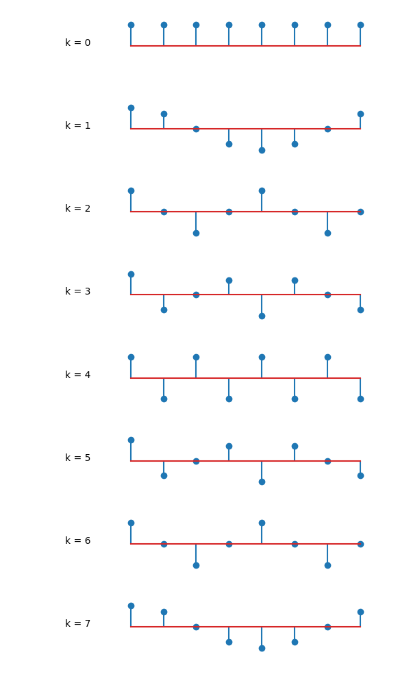
Fig. 3.9 Discrete Harmonics. Shown are the real parts of the complex exponentials \(\phi_k[n] = e^{jk\Omega_0n}\) for \(k=0,\ldots,7\).

Observe that for \(k=0,1,2,3,4\) the frequency is increasing from zero to the maximal frequency exponential \(e^{j\pi n}\) where the value \(x[n]\) jumps from +1 to -1 and back for every \(n\).

The analysis equation in this case is:

\[a_k = \frac{1}{N} \sum_{n=0}^{N-1} x[n] e^{-j k \frac{2\pi}{N} n}\]

For the discrete time Fourier series it is not too hard to derive the analysis equation given the synthesis equation. Let’s start with the synthesis equation and multiply each side with a complex exponential function

\[x[n] e^{-j k' \frac{2\pi}{N} n} = \sum_{k=0}^{N-1} a_k e^{jk\frac{2\pi}{N}n} e^{-j k' \frac{2\pi}{N} n}\]

Now we take the sum over all \(n\) on both sides:

\[\begin{split}\sum_{n=0}^{N-1} x[n] e^{-j k' \frac{2\pi}{N} n} &= \sum_{n=0}^{N-1} \sum_{k=0}^{N-1} a_k e^{jk\frac{2\pi}{N}n} e^{-j k' \frac{2\pi}{N} n}\\ &= \sum_{k=0}^{N-1} a_k \sum_{n=0}^{N-1} e^{j(k-k')\frac{2\pi}{N}n} \\ &= \sum_{k=0}^{N-1} a_k N \delta[k-k']\\ &= N a_{k'}\end{split}\]

and thus:

\[a_{k'} = \frac{1}{N} \sum_{n=0}^{N-1} x[n] e^{-j k' \frac{2\pi}{N} n}\]

In this derivation we have used:

\[\sum_{n=0}^{N-1} e^{j m \frac{2\pi}{N} n} = N\delta[m]\]

Convince yourself that this is true (easily done by plotting the real and imaginary parts of the complex exponential function.

3.4.2. Properties of Discrete Time Fourier Series

Time Domain	Frequency Domain
Synthesis (Inverse Fourier Transform) \[x[n] = \sumN{k} a_k e^{jk \frac{2\pi}{N}n}\]	Analysis (Fourier Transform) \[a_k = \frac{1}{N} \sumN{n} x[n] e^{-j k \frac{2\pi}{N} n}\]
Real Signals \[x[n] \in\setR\]	Symmetry in Fourier transform \[a_{-k} = a_k^\star\]
Even Signals \[x[-n] = x[n]\]	Real Fourier transform \[a_k \text{ is real}\]
Odd Signals \[x[-n] = -x[n]\]	Imaginary Fourier transform \[a_k \text{ is imaginary}\]
Difference \[x[n] - x[n-1]\]	\[(1-e^{-j \frac{2\pi}{N} k})a_k\]
Time Shift \[x[n-n_0]\]	Phase factor \[e^{-j k \frac{1\pi}{N} n_0} a_k\]
Convolution \[x[n] \ast_N y[n] = \sumN{k} x[k] y[n-k]\]	Multiplication \[N a_k b_k\]
Multiplication \[x[n] y[n]\]	Convolution \[\sumN{n} a_n b_{k-n}\]

Real Signals

Let \(x[n]\) be a real valued signal. The analysis equation for \(a_{-k}\) is:

\[a_{-k} = \frac{1}{N} \sum_{n=0}^{N-1} x[n] e^{jk\frac{2\pi}{N} n}\]

and because \(x[n]\) is real we have that

\[a_{-k}^\ast = \frac{1}{N} \sum_{n=0}^{N-1} x[n] e^{-jk\frac{2\pi}{N} n} = a_k\]

Symmetry

Note that the complex exponentials \(e^{j k \frac{2\pi}{N} n\) are periodic with period \(N\) for all \(k\) but then a summation of these exponentials is periodic as well and thus

\[a_{k+N} = a_k\]

or

\[a_{N-k} = a_{-k} = a_k^\star\]

For even \(N\) we have

\[\begin{split}a_0 & \mbox{ is real}\\ a_1 &= a_{N-1}^\star\\ a_2 &= a_{N-2}^\star\\ \vdots\\ a_{N/2} & \mbox{ is real}\\ \vdots\\ a_{N-2} &= a_2^\star\\ a_{N-1} &= a_1^\star\end{split}\]

Synthesis of Real Valued Function

The synthesis equation for \(N\) even is

\[\begin{split}x[n] &= \sum_{k=0}^{N-1} a_k e^{j k \frac{2\pi}{N} n}\\ &= a_0 + \sum_{k=1}^{N/2-1} a_k e^{j k \frac{2\pi}{N} n} + a_{N/2} e^{j\pi n} + \sum_{k=N/2+1}^{N-1} a_k e^{j k \frac{2\pi}{N} n}\\ &= a_0 + \sum_{k=1}^{N/2-1} a_k e^{j k \frac{2\pi}{N} n} + a_{N/2} e^{j\pi n} + \sum_{k=1}^{N/2-1} a_{N-k} e^{j (N-k) \frac{2\pi}{N} n}\\ &= a_0 + \sum_{k=1}^{N/2-1}\left( a_k e^{j k \frac{2\pi}{N} n} + a_{N-k} e^{j (N-k) \frac{2\pi}{N} n}\right) + a_{N/2} e^{j\pi n}\\ &= a_0 + \sum_{k=1}^{N/2-1}\left( a_k e^{j k \frac{2\pi}{N} n} + a_{k}^\star e^{-j k \frac{2\pi}{N} n}\right) + a_{N/2} e^{j\pi n}\end{split}\]

We now write

\[a_k = |a_k| e^{j\angle a_k} \text{ and thus } a_k^\star = |a_k| e^{-j\angle a_k}\]

Leading to

\[\begin{split}x[n] &= a_0 + \sum_{k=1}^{N/2-1}|a_k|\left( e^{j (k \frac{2\pi}{N} n + \angle a_k)} + e^{-j (k \frac{2\pi}{N} n + \angle a_k)} \right) + a_{N/2} e^{j\pi n}\\ &= a_0 + 2 \sum_{k=1}^{N/2-1}|a_k| \cos\left(k \frac{2\pi}{N} n + \angle a_k\right) + a_{N/2} \cos(\pi n)\end{split}\]

3.4.3. Time and Frequency

Both time and frequency are discrete for the DT Fourier Series. Consider the \(k\)-th frequency component corresponding with complex exponential

\[\phi_k[n] = e^{j k \frac{2\pi}{N} n}\]

The radial frequency of this signal is

\[\Omega = k\frac{2\pi}{N}\]

We assume \(N\) is even and thus for \(k=N/2\) we have:

\[k=N/2: \quad \Omega = \pi\]

corresponding with maximal radial frequency that can be represented with the given sampling.

Like in a previous section we can link the radial frequency with the time domain radial frequency \(\w\) and frequency \(f\):

\[\w = \frac{\Omega}{T_s}, \quad f = \frac{\Omega}{2\pi T_s} = \frac{k}{NT_s}\]

where \(T_s\) is the sample time.

The relation between \(n\) and time is simply given as \(t=nT_s\).

Below a plot of the DT function

\[x[n] = 5\sin(2\pi n / N) + \sin(14\pi n / N), \quad n=0,1,\ldots,63\]

and its DT Fourier Transform. Please make sure you understand the plot. You should also be able to plot time on the horizontal axis in the first plot and frequency (in Hz) in the second plot.

Show code for figure

plt.clf()

from DTP import example_timefreq

example_timefreq()
plt.savefig('source/figures/example_timefreq.png')

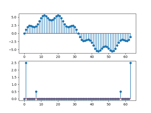
Fig. 3.10 The function \(x[n]\) and its discrete Fourier series.

3.4.4. DTFS in Numpy

Any signal in practice is a discrete time signal but furthermore it is a signal for a finite number of samples. No wonder that the computational way to do frequency analysis is by using the DT Fourier Series.

Unfortunately to add to the confusion the DTFS is known as the Discrete Fourier Transform (DFT) and the fast algorithm to calculate the DFT is called the FFT (Fast Fourier Transform). And even more, the normalization factors are chosen differently than what we used in this section.

In numpy.fft we find that the analysis equation (in the default setting) is:

\[A_k = \sum_{m=0}^{n-1} a_m e^{-2\pi j \frac{mk}{n}}\]

Note the change of notation. The \(A_k\)’s are the Fourier coefficients whereas the \(a_k\)’s are the samples of the signal. Also note that there is no scaling factor in the analysis equation and the \(n\) is the number of samples both in time as well as frequency domain.

The synthesis equation is the inverse DFT:

\[a_m = \frac{1}{n} \sum_{k=0}^{n-1} A_k e^{2\pi j \frac{mk}{n}}\]

Again carefully note the differences with the DT Fourier Series. In the default setting of the FFT in numpy (i.e. parameter norm = ‘backward’) the scaling factors are opposite of what we have used in this chapter (i.e. we have used factor \(1/N\) in the analysis equation and factor \(1\) in the synthesis equation).

As an example let us start with a simple block function

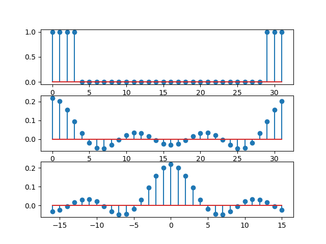
Fig. 3.11 Block function and its discrete Fourier series.

The python code is given below.

def example_DFT_block():
    N = 32
    n = np.arange(32)
    x = np.zeros_like(n)
    x[:4] = 1
    x[-3:] = 1
    fig, axs = plt.subplots(3)
    axs[0].stem(n, x)

    a = fft(x)/N
    axs[1].stem(n, a.real)
    axs[2].stem(n-N//2, np.fft.fftshift(a).real)
    print(n-N//2)

Todo

Code in rst file zetten! Maak de import van fft zichtbaar

3.4.5. DTFS in Linear Algebra Disguise

Look again at the analysis equation. It takes \(N\) numbers \(x[0],\ldots,x[N-1]\) and produces \(N\) complex numbers \(a_0,\ldots,a_{N-1}\). And it does so in a linear fashion meaning that it can be represented as a matrix operation.

Let

\[\begin{split}\v x &= \begin{pmatrix}x[0] & x[1] & \cdots & x[N-1]\end{pmatrix}\T\\ \v a &= \begin{pmatrix}a_0 & a_1 & \cdots & a_{N-1}\end{pmatrix}\T\\ W_N &= e^{-j \frac{2\pi}{N}}\\ F_{kn} &= e^{-j k \frac{2\pi}{N} n} = W_N^{kn}\end{split}\]

then:

\[\v a = \frac{1}{N} F_N \v x\]

The matrix \(F_N\) is called the Fourier matrix.

3.4.6. The Fast Fourier Transform 1

First we start with a simple straightforward implementation of the DFT:

\[A_k = \sum_{m=0}^{N-1} a_m e^{-2\pi j \frac{mk}{N}}\]

Given the signal \(a_m\) (we will follow the numpy fft documentation here) as the vector \(\v a\) we may calculate the DFT coefficients \(A_k\) (in vector \(\v A\)) as:

\[\v A = F \v a\]

where \(F\) is the Fourier matrix with elements \(F_{kn}=W_N^{kn}\). In Python/Numpy the DFT is easy to implement:

def DFT(a):
    """Calculate the DFT of signal `a`"""
    N = len(a)
    n = arange(N)
    W = exp(-1j*2*pi/N)
    F = W**outer(n,n)
    return F @ a

This is indeed what the fft from numpy calculates as well:

from DFT_FFT import DFT
from numpy.fft import fft

a = np.random.random(512)
A1 = DFT(a)
A2 = fft(a)
print(np.allclose(A1,A2))

True

To come up with a faster algorithm for the DFT we rewrite the analysis equation. We assume that \(N\) is some power of \(2\). First we split the sum over the inputs into the even and odd elements:

\[\begin{split}A_k &= \sum_{m=0}^{N-1} a_m e^{-2\pi j \frac{mk}{N}}\\ &= \sum_{m=0}^{N/2-1} a_{2m} e^{-2\pi j \frac{2mk}{N}} + \sum_{m=0}^{N/2-1} a_{2m+1} e^{-2\pi j \frac{(2m+1)k}{N}}\\ &= \sum_{m=0}^{N/2-1} a_{2m} e^{-2\pi j \frac{mk}{N/2}} + e^{-2\pi j k/N} \sum_{m=0}^{N/2-1} a_{2m+1} e^{-2\pi j\frac{mk}{N/2}}\end{split}\]

Note that in the summations over \(m\) runs from \(0\) to \(N/2\), but \(k\) still runs from \(0\) to \(N\). But also note that the exponential \(e^{-2\pi j mk / (N/2)}\) considered as function of \(k\) is periodic with period \(N/2\). So altough both summations in the last equation have to be done for \(k=0,\ldots,N\) we only have to calculate the vasummations for \(k=0,\ldots,N/2\) and repeat these values for larger \(k\)’s. Note that for \(k=0,\ldots,N/2\) the the \(N/2\) values of the first summation are the DFT of the even elements of the input signal and the values in the second summation are the DFT of the odd elements of the input signal. Carefully note that the phase factor \(e^{-2\pi j k/N}\) must be calculated for \(k=0,\ldots,N\).

So we can decompose a DFT of \(N\) samples into two DFT’s of each \(N/2\) samples. But of course a DFT of N/2 samples can be decomposed into two DFT’s of \(N/5\) samples. This leads to the following recursive algorithm:

def FFT(a):
    """
    Calculate the DFT using the FFT (in recursive form)

    Parameters
    ----------
    a : numpy array (n,)
        the signal, len(a) should be power of 2
    """
    N = len(a)
    if N % 2 > 0:
        raise ValueError("Size of a must be a power of 2")
    elif N <= 4:
        return DFT(a)
    else:
        A_even = FFT(a[::2])
        A_odd = FFT(a[1::2])
        factor = exp(-2j * pi * arange(N) / N)
        return concatenate([A_even + factor[:N//2] * A_odd,
                            A_even + factor[N//2:] * A_odd])

Again let’s check if it really works

plt.clf()
from DFT_FFT import FFT
from numpy.fft import fft

a = np.random.random(512)
A1 = FFT(a)
A2 = fft(a)
print(np.allclose(A1,A2))

True

It does work (well this is an \(n=1\) proof, not really a proof but one example where it works..).

Such a recursive implementation as given in this section is certainly not what is used in practice. Recursion is replaced with iteration and the use of many intermediate results is circumvented.

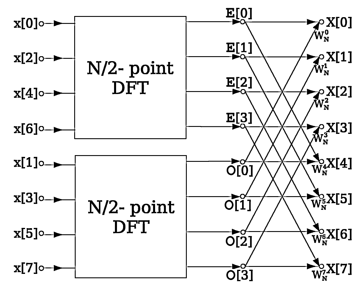
Classically the FFT algorithm is explained in terms of butterflies. Consider the scheme to the right sketching the FFT of a signal \(x[n]\) with \(8\) samples, i.e. \(N=8\). On the even samples we apply of 4 point FFT as well as a 4 point FFT on the odd samples. The 8 values of the DFT \(X[k]\) (again another notation…) of \(X[k]\) are summation of a term of the \(DFT(x_e[n])\) and \(DFT(x_o[n])\), with the contributions from \(DFT(x_o[n])\) multiplied with the complex scaling factor. The way that \(E[0]\) and \(O[0]\) are combined to form \(X[0]\) and \(X[4]\) is called a butterfly; there are thus 4 butterflies in this scheme.

3.4.7. Exercises

1. Discrete Time Periodic Functions

   Given the following signals:

   1. \(x_1[n] = 1 + \cos(\frac{\pi}{4} n)\)

   2. \(x_2[n] = 1 + \cos(\frac{\pi}{4} n) + \sin(\frac{\pi}{2} n)\)

   3. \(x_3[n] = 1 + \cos(\frac{\pi}{3} n) + \cos(\frac{\pi}{2} n)\)

   For each of the signals calculate:

   • The mininal \(N\) such that \(x_i[1],\ldots,x_i[n-1]\) is a periodic signal with period \(N\).

   • The fundamental frequency \(\Omega_0\)

   • The Fourier coefficients \(a_0,\dots,a_{N-1}\)

2. DT Fourier Series

   For each of the functions below (\(N=4\)) calculate the Fourier coefficients. First calculate the Fourier matrix \(F_4\) needed to do the calculation of the Fourier coefficients.

   1. x[n] = {1,2,2,1}

   2. x[n] = {1,0,-1,0}

   3. x[n] = {0,1,1,0}

   4. x[n] = {1,-2,3,-2}

3. Time and Frequency

   In figure Fig. 3.10 a discrete time signal \(x[n]\) is plotted. Redo the figures assuming the discrete signal \(x[n]\) is the sampled version of a continuous time signal \(x(t)\) which is sampled with frequency \(f_s=100 Hz\). In the plot of \(x[n]\) the real time in seconds should be plotted on the horizontal axis and in the plot of the Fourier transform magnitude the horizontal axis should be plotted in Hz.

4. Spectral Leaking

   Consider the Fourier series for \(N=64\). This means that the complex exponentials

   \[\phi_k[n] = e^{j k \frac{2\pi}{N} n}\]

   for \(k=0,\ldots,N-1\) are the basis functions to synthesize all possible frequencies. So as long as the signal \(x[n]\) contains just one of these frequencies we see clear spikes in the DT Fourier series as we have shown in one of the examples in this section.

   Now what happens when you start with a signal

   \[x[n] = \sin((10.5) \frac{2\pi}{N} n)\]

   that has a frequency not exactly represented as a multiple of the fundamental frequency (for this \(N=64\)).

   Plot both \(x[n]\) and the \(a_k\)’s as function of \(k\). Please use the numpy.fft.fft function and take care of the scaling to get from the DFT (fft) to the DT Fourier series. A plot on ‘paper’ (pdf) is enough, i need not see the code.

   What you will see is known as spectral leakage, the peak in the frequency spectrum is not a spike but is broadened in order to synthesize this frequency that is not a multiple of the fundamental frequency.

5. FFT of a Real Signal

   Consider a signal \(a[n]\) with \(2N\) samples where we assume \(N\) is a power of 2. In this (http://www.ti.com/lit/an/spra291/spra291.pdf) note from Texas Intruments it is explained (but not proven) that we calculate the FFT of this real valued signal of \(2N\) samples with a complex valued FFT of just \(N\) sanples.

   Implement their recipe using the FFT algorithm given in this section. Extra points if you can give formal proofs for their recipe.

6. FFT’s in Numpy

   Please read the documentation of the numpy.fft package. There are many FFT algorithms.

   Why is it that their algorithm for the FFT for real values signals only returns an array of length \(N/2+1\) given a real valued array of \(N\) signal samples?

7. Sound Signals

   Reading a wav file in Python/Numpy is easy. Playing it is not so easy… Here we use the librosa package to load sound files. The clarinet sound file can be downloaded here.

   Show code for figure

   plt.clf()
   
   import soundfile
   
   x, sr = soundfile.read('source/Python/Data/clarinet2.wav')
   start = 6000
   N = 1024
   x_frag =  x[start:start+N] # a fragment of the sound signal
   plt.figure(figsize=(10,4))
   plt.plot(x_frag[:256]);
   plt.savefig('source/figures/clarinet.png')
   

   

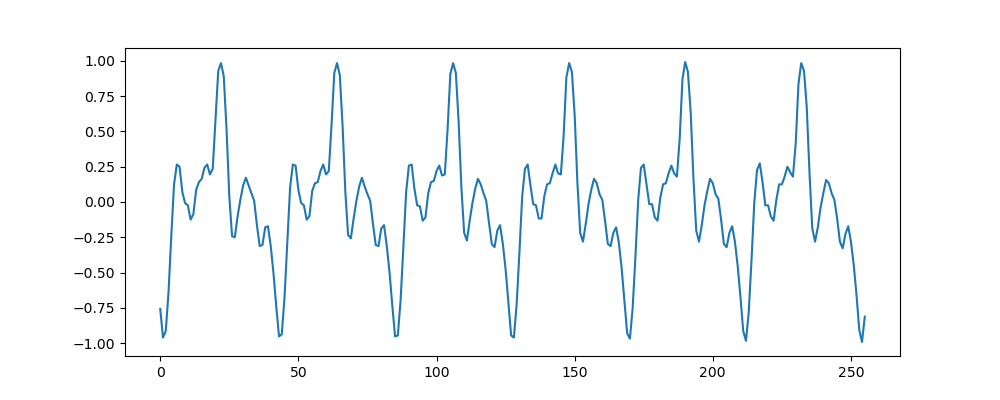
   The fragment is of one note being played on the clarinet. One note of a musical instrument seldomly (never?) corresponds with one frequency in the sound signal. Instead the note corresponds with a fundamental frequency, say \(f_0\), but added to that are the overtones of frequency \(k f_0\) where \(k\) is a positive integer. Not all overtones need to be present and not all are of equal strength. It is the distribution of the energy over all tones that make up the timbre of the instrument.

   1. The fundamental period is visible in the signal plot. Redo the plot but instead of the sample index on the horizontal axis, plot the time.

   2. From this plot calculate the fundamental period and the fundamental frequency in Hz.

   3. Make an FFT of the fragment signal \(x_\text{frag}\) (see code) and plot the magnitude of the frequency response.

      From the plot you can find the fundamental frequency and the overtones. Give the frequencies in Hz of the harmonics (including the fundamental). Compare with your calculation from the time domain plot.

8. Synthesizing Sound

   Create a sound with just four frequencies. Take these to be the fundamental frequency of the clarinet (from the previous exercise) and its three major overtones. Add the sinusoids together each with an amplitude that corresponds with the peak at the frequency of the fundamental of overtones. Also make sure that the relative phases of the 4 sinusoidal waves are in accordance with what you have measured in the previous exercise. Make a signal with the same sample frequency as the clarinet wave file and of about the same duration. You can save the signal as a wav file or you can try to learn Python how to play one (i heard it is easier to do in an IPython notebook).

   Compare, in a qualitative way, the synthesized sound with the real sound of the clarinet.

Footnotes

1

This exposition of the FFT is based on the https://jakevdp.github.io/blog/2013/08/28/understanding-the-fft/