5.3.2. Interpolation

Interpolation is the process of reconstructing a CT signal \(x(t)\) from its samples \(x[n]=x(n T_s)\).

5.3.2.1. Sinc Interpolation

Consider a signal \(x(t)\) that is bandlimited such that \(|X(\omega)|=0\) for \(|\omega|>\omega_b\). We have seen in a previous that in case we sample with frequency \(\omega_s>2\omega_b\) the shifted copies of \(X(\omega)\) do not overlap. So multiplying \(X_s(\omega)\) with a block of width \(\omega_s\) we get \(T_s = \w_s/(2\pi)\) times the Fourier transform of the original signal.

Because multiplication with a block in the Fourier domain corresponds with convolution in the time domain with the inverse Fourier transform of the block.

\[\phi_\infty(t)=T_s\frac{\sin(\w_s/2 t)}{\pi t} \FTright T_s\left(u(\w+\w_s/2) - u(\w-\w_s/2)\right)\]

The proof of this Fourier transform pair is easily done using the inverse Fourier transform:

\[\begin{split}\phi_\infty(t) &= \frac{1}{2\pi} \int_{-\infty}^{\infty} T_s\left( u(\w+\w_s/2) - u(\w-\w_s/2) \right) e^{j\w t} d\w\\ &= \frac{T_s}{2\pi} \int_{-\w_s/2}^{\w_s/2} e^{j\w t} d\w\\ &= \frac{T_s}{2\pi} \frac{1}{j t}\left[e^{j\w t}\right]_{-\w_s/2}^{\w_2/2}\\ &= \frac{T_s}{\pi}\frac{1}{2 j t}\left(e^{j\w_s/2 t}-e^{-j\w_s/2 t}\right)\\ &= \frac{T_s}{\pi}\frac{\sin(\w_s/2 t)}{t} = \frac{\sin(\pi t / T_s)}{\pi t / T_s}\end{split}\]

With \(\phi_{\infty}\) we can calculate \(x(t)\) as:

\[x(t) = (x_s \ast \phi_\infty)(t)\]

Remember that:

\[x_s(t) = \sum_{n=-\infty}^{+\infty} x(n T_s) \delta(t-n T_s)\]

Leading to

\[\begin{split}x(t) &= \int_{-\infty}^{\infty} x_s(t-v) \phi_\infty(v) dv\\ &= \int_{-\infty}^{\infty} \left(\sum_{n=-\infty}^{+\infty} x(n T_s) \delta(t-v-n T_s)\right) \phi_\infty(v) dv\\ &= \sum_{n=-\infty}^{+\infty} x(n T_s) \int_{-\infty}^{\infty} \delta(t-v-n T_s) \phi_\infty(v) dv\\ &= \sum_{n=-\infty}^{+\infty} x(n T_s) \phi_\infty(t-nT_s)\\ &= \sum_{n=-\infty}^{+\infty} x[n] \phi_\infty(t-nT_s)\end{split}\]

Although this looks like a discrete convolution, it is not as \(t\) can take any value. Also note that this is really an interpolation formula in the sense that in case we set \(t=kT_s\) we get \(x(kT_s)=x[k]\) as \(\phi_\infty(kT_s-nT_s)=\delta[k-n]\) due to the fact that the zeros of \(\phi_\infty(t)\) are for \(t=kT_s\) with \(k\not=0\).

The interpolation is illustrated in the figure below.

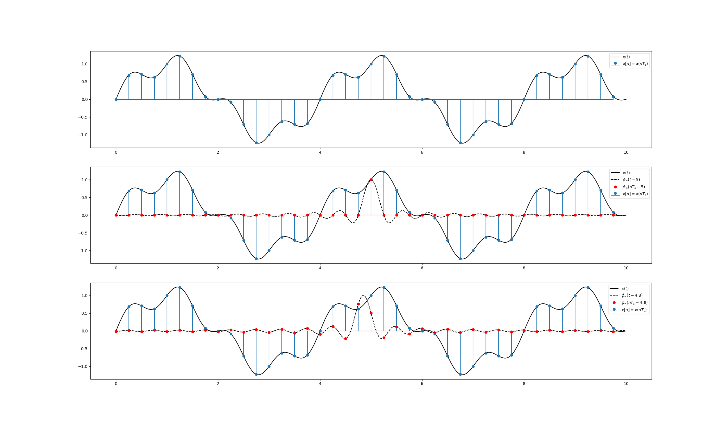
Fig. 5.37 Sampling and Interpolation. At the top the signal \(x(t)\) is shown with the samples \(x[n]=n(nT_s)\). In the middle the sinc interpolation function \(\phi_\infty\) is shown shifted to a sample time. Observe that the values of this shifted sinc function are everywhere zero at the sample points except for the center point where it is equal to one. At the bottom the sinc function is shifted to a position inbetween sample points. Now all sample points will contribute to the interpolated value.